INTRODUCTION

Seismic-scale faults are present in most oil and gas reservoirs. In the shallow crust they are manifested as distinct volumetric entities typically exhibiting complex structures (e.g., Foxford et al., 1998; Davatzes and Aydin, 2003; Shipton et al., 2005; Braathen et al., 2009) and characterized by coupled heterogeneity and anisotropy properties that might enhance flow parallel to faults and impede flow across them (e.g., Antonellini and Aydin, 1994; Shipton et al., 2002; Lampe et al., 2012). Faults that can accommodate long-distance along-fault flow (e.g., because of the presence of stacked entrained host rock bodies) and act as conduits to flow (e.g., because of open, fault-related fractures) are well-documented phenomena. In shallow reservoirs such as in the Champion East field in offshore Brunei Darussalam (van Kessel, 2002) and the Duri field in Indonesia (Waite et al., 1997), faults are affected by very small differential stresses or are even in a tensional stress state. These stress states promote the development of open, fault-related structures (Engelder, 1993; Fossen et al., 2007), and therefore, the corresponding fault zones act as combined baffle–conduit systems to subsurface fluid flow as can be observed at the Casper aquifer, Wyoming (Huntoon and Lundy, 1979); the Cidurian fault, Banten, Indonesia (Fachri and Harsolumakso, 2003); the Roer Valley rift system, central Europe (Bense et al., 2003a, b; Bense and Kooi, 2004; Bense and Van Balen, 2004); the Sandia fault in the Albuquerque basin, United States (Grant, 1982; Haneberg, 1995); the Tensleep sandstone in the Big Horn Basin, United States (Bredehoeft et al., 1992); the Baton Rouge fault, Louisiana (Stoessel and Prochaska, 2005; Bense and Person, 2006); and the Causeway and Goose Point faults, Louisiana (Stoessel and Prochaska, 2005).

Faults in deep reservoirs experiencing critical stress states (e.g., the CS field in Timor gap; Paul et al., 2009), tectonic inversion (e.g., the West Sole field in the southern North Sea; Barr, 2007), and uplift (e.g., the Snøhvit field in the Barents Sea; Wennberg et al., 2008) might also act as dual baffle–conduit systems to fluid flow because they are commonly associated with the formation of open, fault-related fractures. Case studies from the South Eugene Island 330 field in the Gulf of Mexico (Anderson et al., 1994; Roberts et al., 1996; Losh, 1998; Losh et al., 1999; Revil and Cathles, 2002; Haney et al., 2005) provide solid proof of a fault zone acting as a hybrid baffle–conduit system to fluid flow in deep reservoirs. Combined reservoir engineering and time-lapse seismic data and methods used in these studies have been able to detect the ascent of large pulses of overpressured fluid that move at 100 m (328 ft) per year along a growth fault zone (Haney et al., 2005).

In contrast to their volumetric nature, faults in industrial reservoir simulation tools are implemented simply as planes. Within this two-dimensional (2-D) environment, it is common to represent baffle effect of faults on across-fault flow by using fault transmissibility multiplier (FTM) (Manzocchi et al., 1999), whereas flow inside fault zones, particularly in along-dip direction, can be captured implicitly by assigning nonneighbor cell connections using geometrical upscaling (Manzocchi et al., 2008). However, these methods do not perform well for faults that can accommodate voluminous flow and faults that act as conduits to flow described above. In these cases, rendering faults as discrete three-dimensional (3-D) volumetric entities could potentially provide a more accurate model descriptions of flow in reservoir models.

Several reservoir simulation studies that use models with volumetric faults have been carried out to investigate the effect of fault zone multiphase properties (Rivenæs and Dart, 2002; Al-Busafi et al., 2005; Berg and Øian, 2007) and 3-D flow behavior inside fault zones (Flodin et al., 2001; Fredman et al., 2007; Fachri et al., 2011). These studies demonstrate that the combination of volumetric representation of faults and the incorporation of more detailed descriptions of fault zone elements yields a more accurate rendering of fault zone flow properties. These studies, however, use local approaches or small simplified reservoir models to draw their conclusions. Up to now, the effects of volumetric representation of faults on real field-wide flow behavior have remained poorly understood.

In this paper, we first demonstrate a method for incorporating a fault envelope grid on a realistic, field-sized reservoir model used as a tutorial example by a leading reservoir modeling software supplier. We conceptualize the modeled fault zones as a region with dense anastomosing slip zones that bound host rock lenses that are commonly observed in siliciclastic formations with highly porous sandstone layers (e.g., Childs et al., 1996; Foxford et al., 1998). Following previous studies (e.g., Berg and Skar, 2005; Davatzes and Aydin, 2005; Braathen et al., 2009), this region is named as “fault core.” Using fault zone outcrop analogs, lenses and slip zones are described as facies units (Tveranger et al., 2005; Braathen et al., 2009), and their geological and petrophysical properties are populated in the fault envelope grid using combined object-based simulation (e.g., Haldorsen and Damsleth, 1990; Damsleth et al., 1992) and deterministic techniques. The embellished synthetic model is scaled up using flow-based method (King and Mansfield, 1999) to give a volumetric fault (VF) simulation model.

Second, we investigate field-wide flow behaviors and reservoir performances in the VF simulation model by modulating slip zone characteristics: (1) membrane and (2) conduit slip zones. For comparison with the standard method, we generate two FTM reservoir simulation models using (1) membrane and (2) open faults. The models are input to three injection–production schemes: field injection rate (1) smaller than, (2) equal to, and (3) larger than field production rate. This investigation is carried out by analyzing (1) streamline pattern; (2) sweep efficiency; and (3) occurrence, time, and sequence of injected fluid breakthrough.

CONCEPTUAL MODEL OF THICK FAULT CORES IN POROUS SANDSTONE

A fault zone in highly porous sandstone evolves from the formation of an individual deformation band to a cluster of deformation bands and finally a zone of deformation bands and slip surface(s) (Aydin and Johnson, 1978). Slip surface formation is accompanied by the development of slip surface cataclasites along the surface’s walls to form slip zones (Foxford et al., 1998; Tueckmantel et al., 2010). Further process involves an increasing displacement accumulation mainly within a fault core, accommodated by the propagation and linkage of slip surfaces to form first-order lenses and increasing occurrence of fault rocks (Figure 1A) (e.g., Lindanger et al., 2007). During the process, structural overprinting occurs throughout the fault zone (Shipton and Cowie, 2001, 2003; Davatzes and Aydin, 2003; Berg and Skar, 2005).

Figure 1. (A) Drawing and (B) discretization of a cliff outcrop in the Big Hole fault, Utah (A is from Shipton et al., 2005). Slip zones, which in most places bound lenses, are indicated by thick black lines. In B, different colors distinguish different lenses.

Slip zones accommodate most of fault displacement. They consist of various fault rock types, e.g., shale gouge and sandstone cataclasites, and their thickness can range from 1 mm (0.04 in.) to 1 m (3.3 ft) (Foxford et al., 1998). They are commonly continuous and are oriented parallel to subparallel to the main orientation of the fault. The orientation of each slip zone changes gradually along fault strike and fault dip directions, and altogether, slip zone clusters commonly show an anastomosing pattern (Figure 1A) (Childs et al., 1996; Braathen et al., 2009). Normally, one or two continuous main slip zones host significantly larger displacement than the surrounding slip zones.

In many cases, slip zones bound host rock lenses. Such lenses are elongate rock bodies exhibiting various degrees of strain, ranging from undeformed to highly deformed, but commonly can still be recognized as host rock (Foxford et al., 1998). When present, lenses are the volumetric dominant component of a fault core (Braathen et al., 2009). The length of lenses in fault dip direction can range from a few centimeters to more than 100 m (328 ft), whereas their thickness can range from a few centimeters to 50 m (164 ft) (Braathen et al., 2009). Length-to-thickness ratios of sandstone, shale, and limestone lenses ranging from 2:1 to 25:1 have been reported (Berg, 2004; Lindanger et al., 2007; Bastesen et al., 2009; Braathen et al., 2009).

Slip zones are the most important flow domain in a fault zone. They typically have significantly lower permeability than the surrounding lenses and host rock (Sorkhabi and Tsuji, 2005; Tueckmantel et al., 2012) and therefore act as barriers or baffles to across-fault flow. In contrast, they can be in the opening mode because of, e.g., tensional stress state or their critical orientation to compressional stress state in which they could form conduits for along-fault flow (e.g., Antonellini and Aydin, 1994; Shipton et al., 2002).

RESERVOIR SIMULATION MODELS WITH VOLUMETRIC FAULTS

The Fine-Scale Geomodel and Original Reservoir Simulation Grid

The fine-scale geomodel represents a fluvial reservoir (Figure 2A) and approximately measures 6.7 × 6.7 km (4.2 × 4.2 mi) in the horizontal and 700 m (2297 ft) in the vertical. The channel and attached crevasse bodies have good and fair reservoir properties, respectively, and are enclosed within background floodplain deposits with poor reservoir properties. The channel bodies were modeled by implementing strong lateral accretion, and therefore, they have high 3-D connectivity.

Figure 2. (A) The tutorial fine-scale facies model of a channelized reservoir. Injection (I) and production (P) wells are indicated by blue and red lines, respectively. Faults (F) are distinguished by numbers. (B) Map of the reservoir depth at the uppermost layer, which also shows two oil regions (OR). (C) Map of the upscaled porosity model at the uppermost layer.

The geomodel has six normal faults (F1 to F6 in Figure 2A) and one reverse fault (F7 in Figure 2A). Fault F1 cut the whole structure in the north–northwest-south–southeast direction. This fault displaces the reservoir zones completely, leaving no juxtaposed areas, and has the maximum throw of 478 m (1568 ft). Faults F2 to F7 have comparable maximum throw between 35 and 80 m (115 and 263 ft). Faults F2 to F4 intersect with the other faults, whereas F5 to F7 are isolated faults. We consider F1 as the structure-bounding and completely sealing fault. The downthrown part of this fault, which is located much deeper than the oil–water contact, was removed from the grid.

The geomodel contains two structural highs with thick oil columns (Figure 2B), and they are named as (1) oil region 1, located around producer 1 (P1) and producer 2 (P2), and (2) oil region 2, located around producer 3 (P3). The two deepest regions in the southeast and north are the locations of injector 1 (I1) and injector 2 (I2), respectively.

The petrophysical properties of the fine-scale geomodel were scaled up to a reservoir simulation grid (Figure 2C), here named as “original simulation grid” (Figure 3A), which consists of 24 columns, 45 rows, and 7 layers. In average, the grid cell measures 261 × 218 × 6 m (856 × 715 × 20 ft). The total number of cells is approximately 7600, of which approximately 4500 are active cells.

Figure 3. The modeling workflow used in this study. (A) Original simulation grid. (B) Stretched simulation grid. (C) Volumetric fault (VF) simulation grid. (D) Fine-scale geomodel. (E) Coarse fault envelope (FE) grid with upscaled properties. (F) Refined FE grid and displaced property model. (G) VF simulation model. See text for details.

Modeling Workflow and Volumetric Fault Simulation Grid

The workflow to generate a reservoir simulation model that contains volumetric faults is presented in Figure 3. The fault envelope grid was created by following the algorithm proposed by Syversveen et al. (2006) as described in Figure 4. First, based on user-defined fault envelope width, the fault envelope cell stacks in the footwall and hanging wall sides in the original simulation grid (Figure 4A) are delineated (Figure 4B). Second, the following basic steps are executed (Figure 4C–E): (1) stretch the footwall cell stacks in the fault dip direction until their bottom surface aligns with the bottom surface of the hanging wall cell stacks, (2) stretch the hanging wall cell stacks in the fault dip direction until their top surface aligns with the top surface of the footwall cell stacks (black circles and arrows in Figure 4B–E show how steps 1 and 2 are executed), and (3) local grid refinement of the fault envelope grid. These three steps are carried out sequentially throughout the whole fault envelope cell stacks, starting with the cell stacks around fault intersections (Figure 4C, D) and then the rest of the unrefined cell stacks (Figure 4E). Third, after property modeling in the refined fault envelope grid, the fault envelope properties are scaled up into a coarser fault envelope grid (Figure 4F) to ensure that the resulting reservoir simulation model with volumetric faults has a manageable number of cells. Fourth, the upscaled fault envelope grid and properties are merged with the original simulation model as a local grid refinement (Figure 4G).

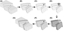Figure 4. Algorithm for creating a reservoir simulation grid that contains a fault envelope grid from (A) a standard corner point grid. (B) Delineate fault cell stacks. (C) Stretch and (D) refine the fault cell stacks around fault intersections. (E) Stretch and refine the remaining fault cell stacks for property modeling. (F) Scale up the fault envelope grid and properties. (G) Merge the fault envelope model with the original corner point grid as a local grid refinement. Based on Syversveen et al. (2006).

In our study, however, we implemented the fault envelope grid as a global grid refinement and only stretched the cells in the footwall blocks (here named as “stretched simulation grid”; Figure 3B). The reasons for taking these decisions are practical. First, to model fault cores we need fine cells only around the grid fault splits, and therefore, nonproportional refinement is required. This facility is not provided by the software for implementing the Syversveen et al. (2006) algorithm. Second, the cell horizontal sizes in the original simulation grid are large, so that fault envelope grid in both footwall and hanging wall, i.e., a situation that would be imposed by using the Syversveen et al. (2006) algorithm, will create extensive regions with unnecessary small cells.

The stretched simulation grid (Figure 3B) was refined nonproportionally in the direction perpendicular to the grid fault segments to complement the grid with a coarse fault envelope grid (coarse FE grids in Figure 3C, E). The fault-perpendicular length of the coarse fault envelope grid was constrained by a field-based relationship between fault throw and fault core thickness (Figure 5). Using the maximum fault throw in the reservoir grid, i.e., 80 m (263 ft), we set the fault-perpendicular length to approximately 10 m (33 ft). The plot of these values falls in the upper range of the data in Figure 5. This cell size selection ensures that most of the fault core lens bodies are included within the fault envelope grid. In regions with thinner fault core, the coarse fault envelope grid covers the fault core and adjacent host rock. Within the fault envelope grid, fault core thicknesses are calculated using the trend function shown in Figure 5.

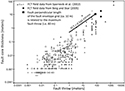Figure 5. Plot of fault throw (FT) versus fault core thickness (FCT). The data points are from faulted sandstone–shale formations in Sinai and Northumberland (Sperrevik et al., 2002) and the Bartlet fault, Utah (Berg and Skar, 2005). The displayed equation was used to calculate FCT in the fault envelop grid.

Neighboring cells around the coarse fault envelope grid were refined nonproportionally in the direction perpendicular to the grid fault segments. To maintain the accuracy of the subsequent flow calculation, the ratios between the fault-perpendicular lengths of the neighboring cells were set between 1 and 3. The resulting reservoir grid, here named as “VF simulation grid” (Figure 3C), consists of 102 columns, 198 rows, and 7 layers. The total number of cells is approximately 141,000, of which approximately 115,000 are active cells.

Refined Fault Envelope Grid

The fine-scale properties (Figure 3D) were scaled up to the VF simulation grid (Figure 3C) to give upscaled properties in all regions including the coarse fault envelope grid (Figure 3E). The resulting fault envelope model was further modified by initially refining the coarse fault envelope grid so that the resulting grid, named as “refined fault envelope grid,” was fine enough to represent typical distribution of fault core lens. This refinement was carried out proportionally but with different refining factors in each axis direction. The chosen cell aspect ratio was constrained by field-based fault core lens data, which show that the average of the ratio between the perpendicular-oriented short axis of lenses (A) and long axis of lenses (C) is 1:9 (Figure 6). For simplicity, we used a slightly different cell aspect ratio, i.e., 1:10.

Figure 6. Plot of the long axis of lenses (C) and the ratio between the long axis and the perpendicular-oriented short axis of lenses (C/A). Data are from Braathen et al. (2009). Black circle indicates the dimension and aspect ratio of the cells of the refined fault envelope grid. n = number of data.

The cell fault-perpendicular length was set to 10 cm (0.3 ft), which is a value in the lower range of the lens thickness data (C axis in Figure 6). Using 1:10 ratio, the cell fault-parallel lengths in the horizontal and vertical directions were set to 1 m (3.3 ft), resulting in a cell dimension of 0.1 × 1 × 1 m (0.3 × 3.3 × 3.3 ft). The plot of the cell dimension and aspect ratio in Figure 6 (black circle) indicates that the cells are smaller than most of the observed natural lenses and hence small enough for modeling them. As another proof, we used the cell size to discretize the outcrop representing our fault core conceptual model (Figure 1A). The resulting discretization, shown in Figure 1B, shows that it captures most of the geometrical complexity of the lenses and hence, the cell dimension is adequate for lens modeling.

With the centimeter-scale average cell dimension, the refined fault envelope grid contains a huge number of cells. This prohibits the creation of the fault envelope grid for the entire field. Instead, the refined fault envelope grid generation, lenses and slip zone modeling, and upscaling were executed fault segment by fault segment.

Fault Core Petrophysical Configuration and Lens Facies Models

Having the refined fault envelope grid, the next step is to predict the petrophysical properties within the grid. In the previous similar studies, this prediction is achieved by the application of fault product distribution factor (Fredman et al., 2008) or displacement function (Fachri et al., 2011) to facies property. In the present study, prior to the application of this function, the fault core thickness was defined using the equation (regression line) shown in Figure 5 and used to separate host rock and fault core parts in the refined fault envelope grid.

Subsequently, within the fault core part, we envisaged that the petrophysical properties configuration was modified because of shear displacement along slip zones. In normal faults (e.g., F2 to F6), from the footwall to hanging wall sides of the fault core, the properties were displaced downward, whereas in reverse faults (F7) the properties were displaced upward. Braathen et al. (2009) show that when slip zones cluster to form fault cores, their density increases toward the hanging wall, and the main slip zone tends to be located at the hanging wall side. These characteristics were implemented in the refined fault envelope model by setting half of the fault displacement to occur along the main slip zone, whereas the other half was distributed linearly in the fault core region hosting other smaller slip zones. The result of this displacement procedure is called “displaced property model” and is shown schematically in Figure 3F.

Simultaneously, the object-based modeling technique (e.g., Haldorsen and Damsleth, 1990; Damsleth et al., 1992) was used to model lenses in the refined fault envelope grid. This technique was selected because it is flexible enough to reproduce the lens characteristics shown in Figures 1 and 6, i.e., (1) highly varied lens dimension and aspect ratio, (2) the presence of single-cell lenses, and (3) the variation in slip zone (lens interface) continuity. To reproduce these characteristics, the following object-based modeling parameters were selected: (1) lensoid object geometry; (2) object dip parallel to the grid pillars (i.e., the fault surfaces); (3) object strike parallel to the fault segments; (4) 1:1:1 object thickness–length–width ratio (in combination with the aspect ratio of the refined envelope grid cell, this corresponds to an object average size of 1 × 10 × 10 m (3.3 × 33 × 33 ft), which is close to the lens average size shown in Figure 6; (5) 99% (very high) object volumetric proportion; and (6) complex object interfaces by enabling the modeled objects to erode each other. Parameters 4 and 5 were combined with the other parameters to avoid too simple object distribution (cf. Fredman et al., 2007; Soleng et al., 2007).

The resulting lens model is shown in Figure 7A (large view) and Figure 7B (detailed view). For model quality control, the lens model (Figure 7B) is compared with the discretized fault core observation using similar scales and observation windows (Figure 1B) (see Fachri et al., 2013a, b for similar model quality control approach). This comparison shows that the important characteristics of the discretized natural lenses described above are reproduced by the model.

Figure 7. (A) Maps and cross sections through the three-dimensional lenses model. (B) Detailed cross-section view of the lenses model. In the fault core regions in A and B, different colors distinguish different lenses. Note that the resulting lenses model resembles the discretized fault core observation (Figure 1B). (C) A combined lenses and slip zone model (here collectively named as merged model) obtained after nonproportional grid refinement and slip zone modeling. This figure is the larger version of the region bounded by the box in B.

Slip Zone Facies and Permeability Models

The lenses are not the most important features controlling fluid flow in the fault core. Slip zones that are typically bounding the lenses and have much smaller size—hence, in a lens-prone fault core they can be seen as the interface between lenses—are features that significantly impede or enhance fluid flow. To represent slip zones in the fault core model, the fault envelope grid was further refined to provide the grid with 1-mm-thick (0.04-in.-thick) cells for representing slip zones discretely. To create these cells in the grid but without having to increase the number of cells too much, a nonproportional refinement was executed. In each axis direction, each parent cell in the fault envelope grid was refined by a factor of two and with a ratio of 1:99 (for fault-perpendicular direction) and 1:999 (for fault-parallel directions). This resulted in a grid with thin (1 mm [0.04 in.]) and thick cells in each axis direction.

Subsequently, slip zone facies was assigned by using the existing lens parameter: if neighboring thick and thin cells host different lens parameter value, indicating that the thin cell is located at the interface between two different lenses, then slip zone facies was assigned to the thin cell. The resulting slip zone network model is shown in Figure 7C.

Permeability values were then deterministically assigned to the slip zone facies. Two slip zone types based on flow characteristics were considered: (1) membrane slip zones, which are slip zones that act as partial barriers to fluid flow; and (2) conduit slip zones, which are slip zones that enhance flow along them and act as partial barriers to flow across them. For each type, we assigned two different permeability sets. Therefore, we have four slip zone permeability models: (1) membrane slip zone with isotropic permeability of 0.001 md, abbreviated as MembraneSZ-0.001md; (2) membrane slip zone with isotropic permeability of 0.01 md, abbreviated as MembraneSZ-0.01md; (3) conduit slip zone with fault-perpendicular permeability of 0.01 md and fault-parallel (strike and dip) permeability of 2000 md, abbreviated as ConduitSZ-2000md; and (4) conduit slip zone with fault-perpendicular permeability of 0.01 md and fault-parallel (strike and dip) permeability of 10,000 md, abbreviated as ConduitSZ-10000md.

Fault Envelope Permeability and Updated Volumetric Fault Simulation Models

Four fine-scale fault envelope petrophysical models were obtained by merging the four slip zone petrophysical models and displaced petrophysical model (Figure 3F). For permeability, all fine-scale fault envelope models were then scaled up using flow-based averaging technique (King and Mansfield, 1999) to give four coarse fault envelope permeability models.

Figure 8 shows the relationships between the upscaled permeabilities of the displaced property models (before the slip zone permeability implementations) and the upscaled permeabilities of the merged models (after the slip zone permeability implementations). Figure 8 reveals the effects of slip zone flow characteristic and permeability on the upscaled permeabilities. Membrane slip zones decrease the upscaled permeabilities, but the effect of increasing slip zone permeability from 0.001 to 0.01 md is very small (compare Figure 8A, C and Figure 8B, D). In each model with membrane slip zones, the fault-parallel permeability (PERMY) (Figure 8B, D) is only slightly higher than the fault-perpendicular permeability (PERMX) (Figure 8A, C).

Figure 8. The relationships between the upscaled permeabilities (PERMX and PERMY) of the displaced property models (before the slip zone permeability implementations) and the upscaled permeabilities of the merged models (after the slip zone permeability implementations) for all slip zone permeability cases: (A and B) MembraneSZ-0.001md case, (C and D) MembraneSZ-0.01md case, (E and F) ConduitSZ-2000md case, and (G and H) ConduitSZ-10000md case. The abbreviations PERMX and PERMY refer to upscaled permeabilities in the directions perpendicular and parallel, respectively, to the corresponding fault segment. In each diagram, circle and triangle symbols indicate that merged model permeabilities are lower and higher than displaced model permeabilities, respectively.

Conduit slip zones increase the upscaled permeabilities in some cells (indicated by triangle data points in Figure 8E–H). The number of cells with increased permeability increases with increasing slip zone permeability (compare Figure 8E, G and Figure 8F, H). In each model with conduit slip zones, the number of cells with increased PERMY (Figure 8F, H) is higher than the number of cells with increased PERMX (Figure 8E, G).

In each model, cells with decreased and lower permeability, i.e., (1) data points below the trend lines in Figure 8A–D and (2) circle data points in Figure 8E–H, are located at the upper and lower parts of the grid. These are the regions in the grid where the fine-scale fault envelope models contain high proportions of impermeable rock originating from the underlying and overlying impermeable layers, respectively (see Figure 3F for comparison).

The four coarse fault envelope models were then used to update the property in the fault envelope grid in the VF simulation models (Figure 3G). This creates (1) two VF simulation models with membrane slip zones and (2) two VF simulation models with conduit slip zones.

RESERVOIR SIMULATION MODELS WITH FAULT TRANSMISSIBLITY MULTIPLIER

For flow simulation comparison to the VF models with membrane slip zones, we generated an FTM model with membrane faults. The fault transmissibility multipliers in this model were estimated using the Manzocchi et al. (1999) algorithm. Two variables required for this estimation are fault permeability and thickness. The fault permeability was calculated using shale gouge ratio, which, in our case, was approximated using shale volume parameter. The fault thickness was calculated by setting the ratio between fault displacement and fault thickness to 170 (Manzocchi et al., 1999).

Similarly, for comparison to the VF models with conduit slip zones, we generated an FTM model with open faults. The FTM in this model was set to 1.

Besides the comparison, the FTM models can be seen as the representations of reservoirs with thin fault cores. In these cases, fluid flow cannot occur inside the fault cores, and flow between two adjacent faulted cells can only occur if they are juxtaposed.

STREAMLINE SIMULATION RESULTS AND DISCUSSION

Streamline simulations were used to investigate flow characteristics and reservoir performance in all FTM models and two end-members of the VF models, i.e., the models with the lowest and highest slip zone permeability: MembraneSZ-0.001md and ConduitSZ-10000md. A streamline is a curve in a 3-D grid along which the velocity vector is a tangent and hence can be viewed as the trajectory of a moving fluid particle in a reservoir. The paths taken by streamlines depend on well locations and injection–production constrains, structure, and reservoir heterogeneity. The details of the algorithm used to generate the streamlines in our study can be found in Pollock (1986).

The model represents an oil field with an oil–water contact at the depth of 1670 m (5479 ft). Table 1 summarizes the fixed dynamic properties used during the streamline simulations. The locations of the water injectors (I1 and I2) and liquid producers (P1, P2, and P3) are shown in Figure 2. The connections between the wells and reservoir were defined in all grid layers. Field water injection rate was set constant to 60,000 m³/day, whereas field liquid production rate was modulated with three cases: (1) field production rate two times larger than the field injection rate, (2) field production rate equal to the field injection rate, and (3) field production rate two times smaller than the field injection rate.

The simulations were run until the longest possible water breakthrough (WBT).

Fluid Flow Characteristics and Sweep Efficiency

The streamlines in all simulated models for the three injection–production schemes are shown in Figure 9. In the FTM model with membrane faults (Figure 9A, E, I), several fault connections can be inferred at the locations where the streamlines can flow across the faults. A notable example is shown by the streamlines from I2 that flow to the nearby fault to the west. The fault connections at these locations make it possible for the injected water to flow directly to the adjacent shallower fault block and therefore sweep the region to the north of P3 (northern oil region 2).

Figure 9. The streamlines in all simulated models for the three injection–production schemes. In each figure, different colors distinguish different streamlines of injector–producer pairs. FTM = fault transmissibility multiplier; I = water injector; OR = oil region; P = liquid producer; SZ = slip zone; VF = volumetric fault.

In the VF model with membrane slip zones (Figure 9B, F, J), however, northern oil region 2 is not swept. Albeit the fault connections still exist, the thick fault cores and I2–P2 configuration subparallel to the nearby fault cores make the water from I2 preferentially flow obliquely inside the fault cores before entering the adjacent shallower fault blocks (cf. Haney et al., 2005, see their figure 1, for similar oblique fluid movement inside a fault zone). As a result, the injected water enters the shallower fault blocks at locations unfavorable for the sweep in northern oil region 2 to occur. Hence, in oil region 2, the VF model with membrane slip zones has poorer sweep efficiency than the FTM model with membrane faults does.

In situations where injector–producer configuration is more perpendicular to the faults, the faults in the FTM model with membrane faults mainly act as baffles to flow. They only allow the injected water to flow between fault blocks at limited fault connections. This causes poor sweep efficiency in oil region 1, as indicated by the low number of streamlines in the region.

On the contrary, the thick fault cores with membrane slip zones act as a combined baffle and conduit system (cf. Fachri et al., 2011). As can be inferred from the streamlines from I1 to P1 and P2 in Figure 9B, F, J, the fault cores divert and at the same time provide pathways for the injected water. The water from I1 is therefore more widely distributed around the faults and sweep thoroughly oil region 1, as indicated by the high number of streamlines in the region.

As in the FTM model with membrane faults, the flow pattern in the FTM model with open faults (Figure 9C, G, K) depends on the number of fault connections. However, because all fault connections do not act as baffles, it is easier for the injected water to flow between fault blocks and sweep oil in the structural highs. Thus, compared with the FTM model with membrane faults and VF model with membrane slip zones, the FTM model with open faults has better sweep efficiency in both oil regions 1 and 2 (compare, e.g., Figure 9A–C).

The flow pattern in the VF model with conduit slip zones is significantly different from those in the other models (compare Figure 9D, H, L to their counterparts). As can be inferred from Figure 8G, H, the conduit slip zones make the thick fault cores act as thief pathways. In Figure 9D, H, a notable example is shown by the streamlines from I1, which, instead of flowing through undeformed highly permeable host rocks between I1 and P3, preferentially flow to the nearby faults to reach the closest producers. Consequently, the injected water from I1 does not sweep southern oil region 2. This is the case where injector distances to two nearby producers are significantly different.

In the case where injector distances to two nearby producers are similar (e.g., I2, P2, and P3), the conduit fault cores provide pathways for the injected water to flow to both producers. This increases the sweep efficiency in the region surrounded by the wells (Figure 9D, H, L). Similar circular streamline patterns around I1–P1, I2–P2, and I2–P3 pairs indicate that sweep efficiency in the VF model with conduit slip zones has less dependency on injector–producer configuration.

Water Breakthrough Occurrence, Time, and Sequence

The WBT occurrence, time, and sequence in all simulated models for the three injection–production schemes are shown in Table 2 and Figure 10. In the FTM model with membrane faults (Figure 10A, E, I), the faults delay WBT. Time to WBT of injector–producer pairs separated by two faults, e.g., I1–P1, are longer than those of injector–producer pairs with similar distance but separated by only one fault, e.g., I2–P2 and I2–P3. As a consequence, water from I1 preferentially flows to P3 and gives early WBT in the producer, although I1–P3 is the injector–producer pair with the longest distance. This also means that the drainage of southern oil region 2 occurs early in the field life. In turn, the early fluid connections through I1–P3 cause significantly late times to WBT between I1–P1 and I1–P2 (considered as no WBT) and hence late full drainage of oil region 1.

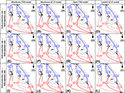Figure 10. Water breakthrough (WBT) occurrence, sequence, and time (in years) in all simulated models for the three injection–production schemes. In each simulation result, each box contains (1) the sequence of WBT occurrence and (2) the time to WBT (in brackets). Red and blue arrows indicate general flow path of water to the production wells from injector 1 (I1) and injector 2 (I2), respectively. FTM = fault transmissibility multiplier; I = water injector; OR = oil region; P = liquid producer; SZ = slip zone; VF = volumetric fault.

In the VF model with membrane slip zones (Figure 10B, F, J), however, the thick fault cores provide partial pathways for the injected water to flow to the nearby producers. Consequently, the number of faults separating injector–producer pairs only slightly affect time to WBT between the pairs. The closest producer–injector pairs, i.e., I1–P1 and I2–P2, show the earliest time to WBT, whereas the longest time to WBT occurs in the producer–injector pairs with the longest distance, i.e., I1–P2 and I1–P3. In addition, the early fluid connections between the closest producer–injector pairs through the fault cores cause very late times to WBT in the producer–injector pairs with the longest distance. Therefore, because sweep efficiencies in oil regions 1 and 2 depend on the producer–injector pairs with the longest distance (i.e., I1–P2 and I1–P3 pairs), the full drainage of these regions occurs very late in the field life.

The WBT sequence in the FTM model with open faults (Figure 10C, G, K) is similar to that in the VF model with membrane slip zones (Figure 10B, F, J). However, in the FTM model with open faults, water can flow more freely between juxtaposed faulted cells, and hence, it shows earlier times to WBT. In addition, because this model has fewer fault connections, the dynamic interplays among the fluid connections of the injector–producer pairs are minimal. Therefore, times to WBT in this model are less varied, and both oil regions 1 and 2 are drained relatively quickly.

Compared with the other models, the VF model with conduit slip zones shows a very different pattern of WBT occurrence (Figure 10D, H, L). The WBT of the injector–producer pairs with shortest distance, e.g., I1–P1, I2–P2, and I3–P3, occurs very early because of thick conduit fault cores. This, in turn, makes it difficult for fluid connections between the injector–producer pairs with the longest distance, e.g., I1–P2 and I1–P3, to occur. Because sweep efficiencies in oil regions 1 and 2 depend on the producer–injector pairs with the longest distance (i.e., I1–P2 and I1–P3 pairs), the full drainage of these regions, depending on injection–production scheme (see the next section), occurs very late in the field life or does not occur at all.

Sensitivity to Injection–Production Scheme and Implications for Field Development Planning

The streamline simulation results show that different models respond differently to the change of injection–production scheme (Figures 9, 10). In the FTM model with membrane faults, the sequence of time to WBT of I1–P1 and I2–P1 is reversed with decreasing field production rate (Figure 10A, E, I), whereas in the other models, WBT sequences are the same for all injection–production schemes. Furthermore, the FTM model with membrane faults shows very similar streamline patterns in all injection–production schemes (Figure 9A, E, I). This suggests that injection–production scheme is not the main cause of the issue in this model, i.e., poor sweep efficiency in oil region 1. A change in I1 location westward (closer to P2) but slightly farther away from the nearby fault might give a better sweep efficiency.

In the VF model with membrane slip zones, the sweep efficiency in oil region 1 decreases when field production rate is lowered (Figure 9B, F, J). Hence, keeping a higher production rate might always be a better option. In contrast, the issue with unswept northern oil region 2 in this model (see Fluid Flow Characteristics and Sweep Efficiency section) persists in all injection–production schemes. A change in I2 placement farther away toward the northwest might give a sweep pattern similar to those in other models. As a more costly but safer alternative to a better sweep in northern oil region 2, another water injector can be added and placed in the same fault block to the north of oil region 2.

Compared with the VF model with membrane slip zones, the FTM model with open faults shows an opposite relationship between sweep efficiency and field production rate. Figure 9C, G, K shows that the sweep efficiency in northern oil region 2 increases when field production rate is lowered, suggesting the use of higher injection rate to develop the field. The good sweep efficiency in both oil regions 1 and 2 shown in Figure 9K suggests that a higher injection rate with the current well placement is an optimal solution for the field development.

Similar to the situation in northern oil region 2 in the FTM model with open faults, the sweep efficiency in the VF model with conduit slip zones increases when field production rate is lowered (Figure 9D, H, L). However, this relationship occurs in a significantly larger region that includes oil region 1 and southern oil region 2 and with the change of injection–production scheme affecting WBT occurrence in some injector–producer pairs (Figure 10D, H, L). Therefore, the use of higher injection rate is required to secure good overall sweep efficiency. Another issue in this model is very late drainage of northern oil region 1 and southern oil region 2 (see the Water Breakthrough Occurence, Time, and Sequence section). This drainage can be accelerated by decreasing the distance of I1–P2 and I1–P3 pairs, e.g., by changing I1 location westward.

Real Case Full-Field Implementation

Because the present study focuses on the effect of slip zone characteristics on field-wide flow behaviors, accurate fault zone representations are not sought. In along-strike and along-dip directions, each fault zone in the present study is assumed to have (1) a simple relationship between fault core thickness and fault throw (Figure 5), (2) constant displacement function type (piecewise linear; Figure 3F), and (3) uniform slip zone characteristics. Natural fault zones, however, show spatial variations in these aspects, and therefore, to be accurate, real case volumetric fault models should capture these variations. Available core data penetrating fault zones and corresponding calculation of missing sections caused by faulting, such as those from the Gullfaks field in the North Sea (Hesthammer and Fossen, 2001, see their figure 4), and fault zone seismic modeling study (e.g., Botter et al., 2014) can help constrain these variations in some locations in fault zones. Starting from these locations, stochastic methods can be used to predict the variations in wider fault zone regions. Fault zone field observations that can be used to predict these variations are few because they need continuous, well-exposed fault zone outcrops. Lunn et al. (2008) is an example of such a study. Their analysis demonstrates that a spatially correlated random field with a spherical covariance structure can be used to describe along-strike fault core thickness variation, which is an important variable for defining fault zone displacement functions. Using this approach, it can be expected that the resulting fault zone models are a combination of thick and thin fault cores and single fault planes. With a stochastic fault zone displacement function completely defined, more accurate displaced property models (cf. Figure 3F) can be generated.

Similarly, slip zone type (baffle or conduit) can be determined using available image data, such as those from the Snøhvit field in the Barents Sea (Wennberg et al., 2008) and well test data (e.g., Aguilera and Ng, 1991). Petrophysical properties from core data penetrating fault zones can be assigned to lens and slip zone facies in merged models (cf. Figure 7C) for the input to flow-based upscaling to obtain final VF simulation models. In the absence of the aforementioned data, slip zone type and properties can be roughly estimated based on four-dimensional seismic, tracer, and production data, which in turn can be used to validate the VF simulation models.

In our synthetic case, for example, only production data are available. The most useful data to crudely estimate fault zone characteristics are the earliest WBT occurrences (Figure 10): (1) early WBT in P2 and relatively late WBT in P3 indicate dominant thin membrane faults, (2) early successive WBTs in P2 and P1 indicate dominant thick fault zones with membrane slip zones, (3) early successive WBTs in P1 and P2 indicate dominant thin open faults, and (4) early WBTs in both P1 and P3 indicate dominant thick fault zones with conduit slip zones. Based on these early WBT occurrence data, the indicated dominant properties can be assigned to volumetric fault regions in the reservoir models, especially those between the analyzed injector–producer pairs. These properties can be assigned based on a detailed modeling study or a database built by using a valid approach (see the next subsection). With this approach, field development can take benefits from the reservoir models with volumetric faults early in the field life.

Efficient Workflow Using Database Approach

The workflow presented in this paper involves many time consuming steps and the implementation of the steps in all coarse fault envelope grid cells. The number of the required steps is even higher for real case implementations such as explained in the previous subsection. A more efficient way to capture the effects of millimeter-scale structural features on fluid flow in the field-scale model is by populating effective permeability in the coarse fault envelope grid after the creation of displaced permeability model (i.e., move forward from Figure 3F to flow-based upscaling to Figure 3G). In this way, the most time-consuming workflow steps, i.e., lens modeling, millimeter-scale gridding, and slip zone modeling in all fault segments, are skipped. This approach, however, requires a thorough database that relates effective permeability of displaced and merged models as described below (see Fachri et al., 2013b, for a similar database approach).

Selected cells in the coarse fault envelope grid related to different fault throws, host rock permeability, and fault configurations are refined so that displaced permeability models can be generated and subsequently used as input for flow-based upscaling to obtain effective permeability of the displaced models. In a real case full-field implementation, these cells are typically those where core data are located (cf. Hesthammer and Fossen, 2001, see their figure 4) or where seismic data can be used to constrain fault configurations (cf. Botter et al., 2014). In parallel, in the same selected cells, the complete workflow (Figure 3) is executed to obtain effective permeability of the merged model. These two parallel procedures give a database with statistical relationships between effective permeability of displaced and merged model. Figure 8 is an example of a small subset of this database. Finally, the complete merged models in all fault envelope grid cells are obtained from the displaced permeability model and the relationships given by the database.

The accuracy of this approach depends on the database quality. The fault envelope cell samples should be representative by taking them from wide ranges of fault throw, host rock permeability, and fault configuration. Once the database is generated, it can be used deterministically by using the correlation coefficients or stochastically by taking into consideration standard deviations using, e.g., sequential Gaussian simulation.

It should be noted that the resulting database is unique to a particular oil and/or gas field because its generation takes into consideration host rock permeability, which is controlled by sedimentary facies and burial and diagenetic histories of the field reservoirs. Therefore, different fields should develop their own database.

Two-Phase Flow Properties of Fault Core Elements

This study has focused on a large-scale flow that occurs in a kilometer-scale reservoir and investigates whether the reservoir simulation results give expected results that can be straightforwardly explained. For this purpose, the use of single-phase flow properties (absolute permeability) and uniform two-phase flow properties (relative permeabilities as functions of water saturation; see Table 1) of fault core elements might be adequate.

When small-scale flow is important for accurate reservoir performance prediction, the use of highly varied two-phase flow properties of fault core elements might be needed. At this scale, slip zones and lenses form a geological arrangement with contrasting porosity and permeability in close proximity (e.g., Shipton et al., 2002; Flodin et al., 2005) and, in turn, assemble a system with short-distance differences in local capillary pressures. This system, under some typical conditions in hydrocarbon production such as recovery through low-rate artificial water injection (e.g., Ringrose et al., 1993) and recoveries through aquifer support and gas expansion (e.g., Al-Busafi et al., 2005; Zijlstra et al., 2007), causes capillary forces to be more dominant than viscous forces in controlling fluid flow. In a fault core with membrane slip zones and hydrocarbon as nonwetting phase, this promotes the trapping and bypassing of hydrocarbon behind the slip zones and, in turn, decreases small-scale reservoir performance (cf. Manzocchi et al., 1998). If small-scale slip zones are considered cumulatively, this effect remains at large-scale reservoir performance (cf. Rivenæs and Dart, 2002).

How these small-scale capillary effects affect the calculation of larger-scale reservoir performance depends on the geometry, relative positions, and relative proportions of the small-scale geological features (e.g., Manzocchi et al., 1998) and the accuracy of two-phase flow property upscaling (e.g., Ringrose et al., 1993). Therefore, accurate 3-D representation of small-scale fault core features in combination with capability to execute straightforward flow simulation in the fine-scale models are imperative when two-phase flow properties of fault core elements are being considered. These combined modeling features, which are not available when using conventional (2-D approach) FTM method (Manzocchi et al., 2002, 2008), have been demonstrated in the previous sections of this paper.

To obtain upscaled two-phase flow properties in the coarse fault envelope cells, the approach presented in the present study can be directly adapted to one of the multiscale modeling methods developed for accurate scaling up of two-phase flow properties of undeformed sedimentary rocks (e.g., Corbett and Jensen, 1993; Ringrose and Corbett, 1994; Pickup et al., 2000). Using this method for a waterflooding in an oil–water system, the millimeter-scale merged models (representing slip zones and lenses) and surrounding larger cells are considered. Each fault core facies in the merged models is assigned unique two-phase flow properties, which currently become more available (e.g., Tueckmantel et al., 2012). Subsequently, waterflooding simulations are carried out with the surrounding larger cells as injection and production cells. Mobility ratio and constant frontal advance rate that are expected to be encountered in the reservoir are used during the simulations. Upscaled absolute permeabilities, relative permeabilities, and capillary pressures of the corresponding coarse fault envelope cells (i.e., the cells occupying the same space as the millimeter-scale merged models) are determined using the Kyte and Berry (1975) equations available in standard reservoir simulator tools.

CONCLUSIONS

The major conclusions of this study can be drawn as follows.

A reliable and accurate modeling of field-sized reservoir with volumetric faults representing fault cores within the framework of the standard reservoir modeling tools can be achieved by using a workflow that involves multipurpose gridding, multiscale modeling and flow-based upscaling, i.e., (1) meter-scale (low-resolution) grids for upscaled fault envelope models and flow simulations; (2) centimeter-scale (medium-resolution) grids (obtained from uniform refinements of the meter-scale grids) for lens models, which can also be seen as representing the distribution of slip zones in fault cores, and displaced property models representing the distribution of petrophysical properties in fault cores; (3) millimeter-scale (high-resolution) grids (obtained from nonuniform refinement of the centimeter-scale grids so that each parent cell contains thin and thick cells) for slip zone implementation in the thin cells and merged models created by combining the slip zone and displaced property models; and (4) flow-based upscaling of petrophysical properties in the merged models to the meter-scale grids.

Fault cores with membrane slip zone clusters act as a dual baffle–conduit system. Injector–producer configuration significantly affects sweep efficiency in reservoirs with these fault cores. Along-strike positioned injector–producer pairs focus flow into the fault cores, decreasing sweep efficiency. Injected fluids of injector–producer pairs positioned to drain perpendicular to the fault cores are partitioned and distributed by the fault cores and therefore increase overall sweep efficiency. The WBT occurrence, time, and sequence in reservoirs with these fault cores are not sensitive to field injection and production rates, whereas sweep efficiency decreases when field production rate is lowered.

Fault cores with conduit slip zone clusters act as thief pathways. Sweep efficiency in reservoirs with these faults has less dependency on injector–producer configuration. The WBT occurrence, time, and sequence in reservoirs with these fault cores are highly sensitive to field injection and production rates, whereas sweep efficiency increases when field production rate is lowered.

The complete modeling workflow presented in this study can be made more efficient by using a database approach. Instead of going through the complete steps in all fault envelope cells, the most time-consuming workflow steps such as millimeter-scale slip zone modeling are carried out only in a selected number of fault envelope cells representative of a wide range of fault throws, host rock permeability, and fault configurations. The result of this procedure is a database with statistical relationships that can be used to populate the remaining fault envelope cells with estimated upscaled permeabilities.

Although this study only considers single-phase flow properties and uniform two-phase flow properties of fault core elements, it provides a complete technical framework for adapting multiscale modeling methods developed for accurate scaling up of two-phase flow properties of undeformed sedimentary rocks.

REFERENCES CITED

Aguilera, R., and M. C. Ng, 1991, Transient pressure analysis of horizontal wells in anisotropic naturally fractured reservoirs: SPE Formation Evaluation, v. 6, p. 95–100, doi:10.2118/19002-PA.
Al-Busafi, B., Q. J. Fisher, and S. D. Harris, 2005, The importance of incorporating the multi-phase flow properties of fault rocks into production simulation models: Marine and Petroleum Geology, v. 22, p. 365–374, doi:10.1016/j.marpetgeo.2004.11.003.
Anderson, R., P. Flemings, S. Losh, J. Austin, and R. Woodhams, 1994, Gulf of Mexico growth fault drilled, seen as oil, gas migration pathways: Oil & Gas Journal, v. 92, no. 23, p. 97–104.
Antonellini, M., and A. Aydin, 1994, Effect of faulting on fluid flow in porous sandstones: Petrophysical properties: AAPG Bulletin, v. 78, no. 3, p. 355–377.
Aydin, A., and A. M. Johnson, 1978, Development of faults as zones of deformation bands and as slip surfaces in sandstones: Pure and Applied Geophysics, v. 116, p. 931–942, doi:10.1007/BF00876547.
Barr, D., 2007, Conductive faults and sealing fractures in the West Sole gas fields, southern North Sea, in Jolley, S. J., D. Barr, J. J. Walsh, and R. J. Knipe, eds., Structurally complex reservoirs: Geological Society, London, Special Publications 2007, v. 292, p. 431–451.
Bastesen, E., A. Braathen, H. Nøttveit, R. H. Gabrielsen, and T. Skar, 2009, Extensional fault cores in micritic carbonate – Case studies from the Gulf of Corinth, Greece: Journal of Structural Geology, v. 31, p. 403–420, doi:10.1016/j.jsg.2009.01.005.
Bense, V. F., and H. Kooi, 2004, Temporal and spatial variations of shallow subsurface temperature as a record of lateral variations in groundwater flow: Journal of Geophysical Research, v. 109, no. B4, B04103.
Bense, V. F., and M. A. Person, 2006, Faults as conduit-barrier systems to fluid flow in siliciclastic sedimentary aquifers: Water Resources Research, v. 42, no. 5, W05421, doi:10.1029/2005WR004480.
Bense, V. F., and R. T. Van Balen, 2004, The effect of fault relay and clay smearing on groundwater flow patterns in the Lower Rhine Embayment: Basin Research, v. 16, p. 397–411, doi:10.1111/j.1365-2117.2004.00238.x.
Bense, V. F., R. T. Van Balen, and J. J. De Vries, 2003a, The impact of faults on the hydrogeological conditions in the Roer Valley Rift System: An overview: Netherlands Journal of Geosciences, v. 82, p. 41–54.
Bense, V. F., E. H. Van den Berg, and R. T. Van Balen, 2003b, Deformation mechanisms and hydraulic properties of fault zones in unconsolidated sediments; the Roer Valley Rift System: The Netherlands: Hydrogeology Journal, v. 11, p. 319–332, doi:10.1007/s10040-003-0262-8.
Berg, S. S., 2004, The architecture of normal fault zones in sedimentary rocks: Analyses of fault core composition, damage zone asymmetry, and multi-phase flow properties, Ph.D. thesis, University of Bergen, Bergen, Norway, 118 p.
Berg, S. S., and E. Øian, 2007, Hierarchical approach for simulating fluid flow in normal fault zones: Petroleum Geoscience, v. 13, p. 25–35, doi:10.1144/1354-079305-676.
Berg, S. S., and T. Skar, 2005, Controls on damage zone asymmetry of a normal fault zone: Outcrop analyses of a segment of the Moab fault, SE Utah: Journal of Structural Geology, v. 27, p. 1803–1822, doi:10.1016/j.jsg.2005.04.012.
Botter, C., N. Cardozo, S. Hardy, I. Lecomte, and A. Escalona, 2014, From mechanical modeling to seismic imaging of faults: A synthetic workflow to study the impact of faults on seismic: Marine and Petroleum Geology, v. 57, p. 187–207, doi:10.1016/j.marpetgeo.2014.05.013.
Braathen, A., J. Tveranger, H. Fossen, T. Skar, N. Cardozo, S. Semshaug, E. Bastesen, and E. Sverdrup, 2009, Fault facies and its application to sandstone reservoirs: AAPG Bulletin, v. 93, no. 7, p. 891–917, doi:10.1306/03230908116.
Bredehoeft, J. D., K. Belitz, and S. Sharp-Hansen, 1992, The hydrodynamics of the Big Horn Basin: A study of the role of faults: AAPG Bulletin, v. 76, no. 4, p. 530–546.
Childs, C., A. Nicol, J. Walsh, and J. Watterson, 1996, Growth of vertically segmented normal faults: Journal of Structural Geology, v. 18, p. 1389–1397, doi:10.1016/S0191-8141(96)00060-0.
Corbett, P. W., and J. L. Jensen, 1993, Application of probe permeametry to the prediction of two-phase flow performance in laminated sandstones (lower Brent Group, North Sea): Marine and Petroleum Geology, v. 10, p. 335–346, doi:10.1016/0264-8172(93)90078-7.
Damsleth, E., C. B. Tjolsen, H. Omre, and H. H. Haldorsen, 1992, A two-stage stochastic model applied to a North Sea reservoir: Journal of Petroleum Technology, v. 44, p. 402–486, doi:10.2118/20605-PA.
Davatzes, N. C., and A. Aydin, 2003, Overprinting faulting mechanisms in high porosity sandstones of SE Utah: Journal of Structural Geology, v. 25, p. 1795–1813, doi:10.1016/S0191-8141(03)00043-9.
Davatzes, N. C., and A. Aydin, 2005, Distribution and nature of fault architecture in a layered sandstone and shale sequence: An example from the Moab fault, Utah, in Sorkhabi, R., and Y. Tsuji, eds., Faults, fluid flow, and petroleum traps: AAPG Memoir 85, p. 153–180.
Engelder, J. T., 1993, Stress regimes in the lithosphere: Princeton, New Jersey, Princeton University Press, 492 p.
Fachri, M., and A. H. Harsolumakso, 2003, Structural geology and lateral boundaries of Jakarta Groundwater Basin: Buletin Geologi, v. 35, no. 3, p. 91–106.
Fachri, M., A. Rotevatn, and J. Tveranger, 2013a, Fluid flow in relay zones revisited: Towards an improved representation of small-scale structural heterogeneities in flow models: Marine and Petroleum Geology, v. 46, p. 144–164, doi:10.1016/j.marpetgeo.2013.05.016.
Fachri, M., J. Tveranger, A. Braathen, and S. Schueller, 2013b, Sensitivity of fluid flow to deformation-band damage zone heterogeneity: A study using fault facies and truncated Gaussian simulation: Journal of Structural Geology, v. 52, p. 60–79, doi:10.1016/j.jsg.2013.04.005.
Fachri, M., J. Tveranger, N. Cardozo, and Ø. Pettersen, 2011, The impact of fault envelope structures on fluid flow: A screening study using fault facies: AAPG Bulletin, v. 95, no. 4, p. 619–648, doi:10.1306/09131009132.
Flodin, E. A., A. Aydin, L. J. Durlofski, and B. Yeten, 2001, Representation of fault zone permeability in reservoir flow models: SPE Annual Technical Conference and Exhibition, New Orleans, Louisiana, September 30–October 3, 2001, SPE-71617-MS, 10 p., doi:10.2118/71617-MS.
Flodin, E. A., M. Gerdes, A. Aydin, and W. D. Wiggins, 2005, Petrophysical properties of cataclastic fault rock in sandstone, in Sorkhabi, R., and Y. Tsuji, eds., Faults, fluid flow, and petroleum traps: AAPG Memoir 85, p. 197–217.
Fossen, H., R. A. Schultz, Z. K. Shipton, and K. Mair, 2007, Deformation bands in sandstones: A review: Journal of Geological Society, v. 164, no. 4, p. 755–769.
Foxford, K. A., J. J. Walsh, J. Watterson, I. R. Garden, S. C. Guscott, and S. D. Burley, 1998, Structure and content of the Moab Fault Zone, Utah, USA, and its implications for fault seal prediction, in Jones, G., Q. J. Fisher, and R. J. Knipe, eds., Faulting, fault sealing and fluid flow in hydrocarbon reservoirs: Geological Society, London, Special Publications 1998, v. 147, p. 87–103.
Fredman, N., J. Tveranger, N. Cardozo, A. Braathen, H. H. Soleng, P. Røe, A. Skorstad, and A. R. Syversveen, 2008, Fault facies modelling: Technique and approach for 3-D conditioning and modelling of faulted grids: AAPG Bulletin, v. 92, no. 11, p. 1457–1478, doi:10.1306/06090807073.
Fredman, N., J. Tveranger, S. L. Semshaug, A. Braathen, and E. Sverdrup, 2007, Sensitivity of fluid flow to fault core architecture and petrophysical properties of fault rocks in siliciclastic reservoirs: A synthetic fault model study: Petroleum Geoscience, v. 13, p. 305–320, doi:10.1144/1354-079306-721.
Haldorsen, H. H., and E. Damsleth, 1990, Stochastic modeling: Journal of Petroleum Technology, v. 42, p. 404–412, doi:10.2118/20321-PA.
Haney, M. M., R. Snieder, J. Sheiman, and S. Losh, 2005, A moving fluid pulse in a fault zone: Nature, v. 437, no. 7055, p. 46–49, doi:10.1038/437046a.
Haneberg, W. C., 1995, Steady state groundwater flow across idealized faults: Water Resources Research, v. 31, p. 1815–1820, doi:10.1029/95WR01178.
Hesthammer, J., and H. Fossen, 2001, Structural core analysis from the Gullfaks area, northern North Sea: Marine and Petroleum Geology, v. 18, p. 411–439, doi:10.1016/S0264-8172(00)00068-4.
Huntoon, P. W., and D. A. Lundy, 1979, Fracture-controlled ground-water circulation and well siting in the vicinity of Laramie, Wyoming: Groundwater, v. 17, p. 463–469, doi:10.1111/j.1745-6584.1979.tb03342.x.
Grant, P. R., 1982, Geothermal potential in the Albuquerque area, New Mexico: Albuquerque Country II: New Mexico Geological Society Guidebook, v. 33, p. 325–332.
King, M. J., and M. Mansfield, 1999, Flow simulation of geologic models: SPE Reservoir Evaluation & Engineering, v. 2, p. 351–367, doi:10.2118/57469-PA.
Kyte, J. R., and D. W. Berry, 1975, New pseudo functions to control numerical dispersion: SPE Journal, v. 15, p. 269–276, doi:10.2118/5105-PA.
Lampe, C., G. Song, L. Cong, and X. Mu, 2012, Fault control on hydrocarbon migration and accumulation in the Tertiary Dongying depression, Bohai Basin, China: AAPG Bulletin, v. 96, no. 6, p. 983–1000, doi:10.1306/11031109023.
Lindanger, M., R. H. Gabrielen, and A. Braathen, 2007, Analysis of rock lenses in extensional faults: Norwegian Journal of Geology, v. 87, p. 361–372.
Losh, S., 1998, Oil migration in a major growth fault: Structural analysis of the pathfinder core, South Eugene Island block 330, offshore Louisiana: AAPG Bulletin, v. 82, no, 9, p. 1694–1710.
Losh, S., L. Eglinton, M. Schoell, and J. Wood, 1999, Vertical and lateral fluid flow related to a large growth fault, South Eugene Island Block 330 Field, offshore Louisiana: AAPG Bulletin, v. 83, no. 2, p. 244–276.
Lunn, R. J., Z. K. Shipton, and A. M. Bright, 2008, How can we improve estimates of bulk fault zone hydraulic properties?, in Wibberley, C. A. J., W. Kurz, J. Imber, R. E. Holdsworth, and C. Collettini, eds., The internal structure of fault zones: Implications for mechanical and fluid-flow properties: Geological Society, London, Special Publications 2008, v. 299, p. 231–237.
Manzocchi, T., A. E. Heath, B. Palananthakumar, C. Childs, and J. J. Walsh, 2008, Faults in conventional flow simulation models: A consideration of representational assumptions and geological uncertainties: Petroleum Geoscience, v. 14, p. 91–110, doi:10.1144/1354-079306-775.
Manzocchi, T., A. E. Heath, J. J. Walsh, and C. Childs, 2002, The representation of two phase fault-rock properties in flow simulation models: Petroleum Geoscience, v. 8, p. 119–132, doi:10.1144/petgeo.8.2.119.
Manzocchi, T., P. S. Ringrose, and J. R. Underhill, 1998, Flow through fault systems in high-porosity sandstones, in Coward, M. P., T. S. Daltaban, and H. Johnson, eds., Structural geology in reservoir characterization: Geological Society, London, Special Publications 1998, v. 127, p. 65–82.
Manzocchi, T., J. J. Walsh, P. Nell, and G. Yielding, 1999, Fault transmissibility multipliers for flow simulation models: Petroleum Geoscience, v. 5, p. 53–63, doi:10.1144/petgeo.5.1.53.
Paul, P. K., M. D. Zoback, and P. H. Hennings, 2009, Fluid flow in a fractured reservoir using a geomechanically constrained fault-zone-damage model for reservoir simulation: SPE Reservoir Evaluation & Engineering, v. 12, p. 562–575, doi:10.2118/110542-PA.
Pickup, G., P. S. Ringrose, and A. Sharif, 2000, Steady-state upscaling: From lamina-scale to full-field model: SPE Journal, v. 5, p. 208–217, doi:10.2118/62811-PA.
Pollock, D. W., 1986, Semi-analytical computational of path lines for finite difference models: Groundwater, v. 26, p. 743–750, doi:10.1111/j.1745-6584.1988.tb00425.x.
Revil, A., and L. M. Cathles, 2002, Fluid transport by solitary waves along growing faults: A field example from the South Eugene Island Basin, Gulf of Mexico: Earth and Planetary Science Letters, v. 202, p. 321–335, doi:10.1016/S0012-821X(02)00784-7.
Ringrose, P. S., and P. W. M. Corbett, 1994, Controls on two-phase fluid flow in heterogeneous sandstones, in J. Parnell, ed., Geofluids: Origin, migration and evolution of fluids in sedimentary basin: Geological Society, London, Special Publications 1994, v. 78, p. 141–150.
Ringrose, P. S., K. S. Sorbie, P. W. M. Corbett, and J. L. Jensen, 1993, Immiscible flow behaviour in laminated and cross-bedded sandstones: Journal of Petroleum Science Engineering, v. 9, p. 103–124, doi:10.1016/0920-4105(93)90071-L.
Rivenæs, J. C., and C. Dart, 2002, Reservoir compartemantelization by water-saturated faults – Is evaluating possible with today’s tools?, in A. G. Koestler and R. Hunsdale, eds., Hydrocarbon seal quantification: Norwegian Petroleum Society Special Publication 11, p. 173–186, doi:10.1016/S0928-8937(02)80014-5.
Roberts, S. J., J. A. Nunn, L. M. Cathles, and F.-D. Cipriani, 1996, Expulsion of abnormally pressured fluids along faults: Journal of Geophysical Research, v. 101, no. B12, p. 28231–28252, doi:10.1029/96JB02653.
Shipton, Z. K., and P. A. Cowie, 2001, Analysis of three-dimensional damage zone development over a micron to km scale range in the high-porosity Navajo sandstone, Utah: Journal of Structural Geology, v. 23, p. 1825–1844, doi:10.1016/S0191-8141(01)00035-9.
Shipton, Z. K., and P. A. Cowie, 2003, A conceptual model for the origin of fault damage zone structures in high-porosity sandstone: Journal of Structural Geology, v. 25, p. 333–344, doi:10.1016/S0191-8141(02)00037-8.
Shipton, Z. K., J. P. Evans, K. Robeson, C. B. Forster, and S. Snelgrove, 2002, Structural heterogeneity and permeability in faulted eolian sandstone: Implications for subsurface modeling of faults: AAPG Bulletin, v. 86, no. 5, p. 863–883.
Shipton, Z. K., J. P. Evans, and L. B. Thompson, 2005, The geometry and thickness of deformation-band fault core and its influence on sealing characteristics of deformation-band fault zones, in R. Sorkhabi and Y. Tsuji, eds., Fault, fluid flow, and petroleum trap: AAPG Memoir 85, p. 181–195.
Soleng, H., A. R. Syversveen, A. Skorstad, and J. Tveranger, 2007, Flow through inhomogeneous fault zones: Society of Petroleum Engineers Annual Technical Conference and Exhibition, Anaheim, California, November 11–14, 2007, SPE-110331-MS, 7 p., doi:10.2118/110331-MS.
Sorkhabi, R., and Y. Tsuji, 2005, The place of faults in petroleum traps, in R. Sorkhabi and Y. Tsuji, eds., Fault, fluid flow, and petroleum trap: AAPG Memoir 85, p. 1–31.
Sperrevik, S., P. A. Gillespie, J. F. Quentin, T. Halvorsen, and R. J. Knipe, 2002, Empirical estimation of fault rock properties, in A. G. Koestler and R. Hunsdale, eds., Hydrocarbon seal quantification: Norwegian Petroleum Society Special Publication 11, p. 109–125, doi:10.1016/S0928-8937(02)80010-8.
Stoessel, R. K., and L. Prochaska, 2005, Chemical evidence for migrating of deep formation fluids into shallow aquifers in South Louisiana: Gulf Coast Association of Geological Societies Transactions, v. 55, p. 794–808.
Syversveen, A. R., A. Skorstad, H. H. Soleng, P. Røe, and J. Tveranger, 2006, Facies modelling in fault zones: Proceedings of the 10th European Conference on the Mathematics of Oil Recovery, Amsterdam, Netherlands, September 4–7, 2006, 9 p.
Tueckmantel, C., Q. J. Fisher, C. A. Grattoni, and A. C. Aplin, 2012, Single- and two-phase fluid flow properties of cataclastic fault rocks in porous sandstone: Marine and Petroleum Geology, v. 29, p. 129–142, doi:10.1016/j.marpetgeo.2011.07.009.
Tueckmantel, C., Q. J. Fisher, R. J. Knipe, H. Lickorish, and S. M. Khalil, 2010, Fault seal prediction of seismic-scale normal faults in porous sandstones: A case study from the eastern Gulf of Suez rift, Egypt: Marine and Petroleum Geology, v. 27, p. 334–350, doi:10.1016/j.marpetgeo.2009.10.008.
Tveranger, J., A. Braathen, T. Skar, and A. Skauge, 2005, Centre for integrated petroleum research—Research activities with emphasis on fluid flow in fault zones: Norwegian Journal of Geology, v. 85, p. 63–71.
van Kessel, O., 2002, Champion East: Low-cost redevelopment of shallow, stacked, and faulted heavy-oil reservoirs: SPE Reservoir Evaluation & Engineering, v. 5, p. 295–301, doi:10.2118/78674-PA.
Waite, M. W., R. Sigit, A. V. Rusdibiyo, T. Susanto, H. Primadi, and D. Satriana, 1997, Application of seismic monitoring to manage an early-stage steamflood: SPE Reservoir Engineering, v. 12, p. 277–283, doi:10.2118/37564-PA.
Wennberg, O. P., O. Malm, T. Needham, E. Edwards, S. Ottesen, F. Karlsen, L. Rennan, and R. Knipe, 2008, On the occurrence and formation of open fractures in the Jurassic reservoir sandstones of the Snøhvit Field, SW Barents Sea: Petroleum Geoscience, v. 14, p. 139–150, doi:10.1144/1354-079308-739.
Zijlstra, E. B., P. H. M. Reemst, and Q. J. Fisher, 2007, Incorporation of fault properties into production simulation models of Permian reservoirs from the southern North Sea, in Jolley, S. J., D. Barr, J. J. Walsh, and R. J. Knipe, eds., Structurally complex reservoirs: Geological Society, London, Special Publications 2007, v. 292, p. 295–308, doi:10.1144/SP292.17.
AUTHORS
Muhammad Fachri is a senior geoscientist at ARA Petroleum. He received his B.Sc. degree in geophysics in 1999 and M.Sc. degree in structural geology in 2002 from the Institute Technology Bandung. In 2014 he received his Ph.D. in reservoir modeling from the University of Bergen. Before joining ARA Petroleum, he worked for Weatherford Petroleum Consultants and Statoil. His research interests include faults, their implementation in reservoir models, and fault zone fluid flow.
Jan Tveranger received his Dr. Scient. from the University of Bergen in 1995. He worked for Saga Petroleum and later Norsk Hydro before becoming head of the geoscience group at the Centre for Integrated Petroleum Research. He currently holds an adjunct professorship of geomodeling at the Department of Earth Science, University of Bergen.
Alvar Braathen received his Dr. Scient. degree from the University of Tromsø, Norway, in 1994. Subsequently, he worked for the Geological Survey of Norway, the Centre for Integrated Petroleum Research at the University of Bergen, and the University Centre in Svalbard (UNIS), Norway, before being appointed professor in structural geology at the Department of Geosciences, University of Oslo. He holds an adjunct professorship at UNIS.
Per Røe received his siv. ing. degree in industrial mathematics from Norges Teknisk-Naturvitenskapelige Universitet in 2001. He has worked as a research scientist at the Norwegian Computing Center since 2002 and since 2005 has mainly worked with uncertainty modeling related to geological features with a focus on the modeling of geological faults.
ACKNOWLEDGMENTS
The research was carried out as part of the Fault Facies Project at Uni Research Centre for Integrated Petroleum Research, University of Bergen, Norway. The Research Council of Norway, StatoilHydro (now Statoil), and ConocoPhillips are thanked for financial support to this research. The paper has benefited from constructive reviews by M. E. Meurer and two anonymous reviewers. Roxar Software Solutions (now Emerson Process Management) is acknowledged for the provision of academic licenses for the Roxar RMS. Dongfang Qu and consulting geologist Frances Plants Whitehurst gave input on technical and editorial issues, which led to further improvement of the paper.