The AAPG/Datapages Combined Publications Database
AAPG Bulletin
Full Text
![]() Click to view page images in PDF format.
Click to view page images in PDF format.
AAPG Bulletin, V.
DOI: 10.1306/05111817249
Hydrocarbon prospectivity of the Cooper Basin, Australia
Lisa S. Hall,1 Tehani J. Palu,2 Andrew P. Murray,3 Christopher J. Boreham,4 Dianne S. Edwards,5 Anthony J. Hill,6 and Alison Troup7
1Geoscience Australia, Symonston, Australian Capital Territory, Australia; [email protected]
2Geoscience Australia, Symonston, Australian Capital Territory, Australia; [email protected]
3Murray Partners PPSA Pty. Ltd., Perth, Western Australia, Australia; [email protected]
4Geoscience Australia, Symonston, Australian Capital Territory, Australia; [email protected]
5Geoscience Australia, Symonston, Australian Capital Territory, Australia; [email protected]
6Department of the Premier and Cabinet, Adelaide, South Australia, Australia; [email protected]
7Department of Natural Resources and Mines, Geological Survey of Queensland, Brisbane, Queensland, Australia; [email protected]
ABSTRACT
The Pennsylvanian–Middle Triassic Cooper Basin is Australia’s premier conventional onshore hydrocarbon-producing province. The basin also hosts a range of unconventional gas play types, including basin-centered gas and tight gas accumulations, deep dry coal gas associated with the Patchawarra and Toolachee Formations, and the Murteree and Roseneath shale gas plays.
This study used petroleum systems analysis to investigate the maturity and generation potential of 10 Permian source rocks in the Cooper Basin. A deterministic petroleum systems model was used to quantify the volume of expelled and retained hydrocarbons, estimated at 1272 billion BOE (512 billion bbl and 760 billion BOE) and 977 billion BOE (362 billion bbl and 615 billion BOE), respectively. Monte Carlo simulations were used to quantify the uncertainty in volumes generated and to demonstrate the sensitivity of these results to variations in source-rock characteristics.
The large total generation potential of the Cooper Basin and the broad distribution of the Permian source kitchen highlight the basin’s significance as a world-class hydrocarbon province. The large disparity between the calculated volume of hydrocarbons generated and the volume so far found in reservoirs indicates the potential for large volumes to remain within the basin, despite significant losses from leakage and water washing. The hydrocarbons expelled have provided abundant charge to both conventional accumulations and to the tight and basin-centered gas plays, and the broad spatial distribution of hydrocarbons remaining within the source rocks, especially those within the Toolachee and Patchawarra Formations, suggests the potential for widespread shale and deep dry coal plays.
INTRODUCTION
The Pennsylvanian–Middle Triassic Cooper Basin is located in northeastern South Australia and southwestern Queensland. It is Australia’s premier onshore hydrocarbon-producing province and supplies large volumes of gas to the eastern Australian gas market. As of December 2014, the total identified resources (remaining identified and produced) in the Cooper and Eromanga Basins included 447 million bbl (71 GL) of oil, 160 million bbl of condensate (25 GL), 220 million bbl (36 GL) of liquefied petroleum gas, and 10.2 tcf (0.29 Tm3) of gas (Australian Energy Resources Assessment, 2017). The basin also hosts a range of unconventional gas play types within the Permian Gidgealpa Group, including basin-centered and tight gas accumulations within the Patchawarra, Toolachee, Epsilon, and Daralingie Formations, deep dry coal gas associated with the Patchawarra and Toolachee Formations, the Murteree and Roseneath shale gas plays, and coal seam gas from the Patchawarra Formation in the Weena trough (Goldstein et al., 2012; Geoscience Australia, 2017a; Dunlop et al., 2017). The principal source rocks for both conventional and unconventional accumulations are the Permian coals, coaly shales, and shales of the Gidgealpa Group (Boreham and Hill, 1998; Deighton et al., 2003; Hall et al., 2016a).
Although the Cooper Basin is a mature exploration province, the ultimate potential of the basin and the remaining undiscovered hydrocarbons present are still poorly defined. In addition, most of the new production from unconventional petroleum systems is underpinned by a data set generated from exploitation of the corresponding conventional systems. To address these issues and to highlight any overlooked exploration opportunities, a regional study of the petroleum system was required to better understand the total volume of hydrocarbons generated from each source rock, the volumes of migrated hydrocarbons, and the volume remaining in or near the source beds for potential stimulated production.
This study used petroleum systems analysis (PSA) to quantify the spatial distribution and petroleum generation potential of Permian source rocks across the Cooper Basin. A three-dimensional (3-D) basin model, characterizing the regional basin architecture (Hall et al., 2015), was used to provide the framework for a pseudo-3-D petroleum systems model (Hall and Palu, 2016). Source-rock characteristics (distribution, amount, and quality) were assigned to the model based on an extensive review of well, wire-line log, and source-rock geochemical data (Hall et al., 2016a). Petroleum systems modeling results, incorporating the recently published source-specific kinetics of Mahlstedt et al. (2015), highlight the variability in burial, thermal, and hydrocarbon generation histories for each source rock across the basin (Hall et al., 2015, 2016c). Migration, fluid properties, and geochemical correlation of fluids to source were not part of this study, although a summary and some general comments on these subjects are included in the Discussion section.
The PSA results provide a regional framework for understanding the remaining conventional and unconventional hydrocarbon prospectivity of the basin and highlight the relative importance of the different unconventional play types.
BASIN GEOLOGY
Tectonic Setting
The Cooper Basin is a Pennsylvanian–Middle Triassic intracratonic basin that covers an area of approximately 127,000 km2 (∼49,035 mi2) and reaches a maximum depth of more than 4400 m (14,438 ft; Figure 1; Gravestock et al., 1998; Draper, 2002; McKellar, 2013; Carr et al., 2016). It unconformably overlies the lower Paleozoic Warburton Basin in the southwest and Devonian Warrabin trough and Barrolka depression in the northeast (Gravestock et al., 1998; Draper et al., 2004).
 Figure 1. Cooper Basin location map. Basin outline from Stewart et al. (2013). JNP = Jackson–Naccowlah–Pepita; NSW = New South Wales; PSA = petroleum systems analysis; QLD = Queensland; SA = South Australia.
The Cooper Basin is entirely and disconformably overlain by the Jurassic–Cretaceous Eromanga Basin, which reaches more than 2500 m (8202 ft) thick over the Cooper Basin (Gravestock et al., 1998; Cook et al., 2013; Stewart et al., 2013). Overlying the Eromanga Basin is the Paleocene to Quaternary Lake Eyre Basin; however, this is less than 300 m (984 ft) thick over the Cooper Basin (Ransley and Smerdon, 2012; Cook and Jell, 2013). The Eromanga and Eyre Basins contain the extensive groundwater system of the Great Artesian Basin (e.g., Ransley and Smerdon, 2012).
The depositional phases of the Cooper, Eromanga, and Eyre Basins were driven by regional tectonic activity along the convergent eastern Australian plate margin (e.g., Gallagher, 1988; Korsch and Totterdell, 2009; Korsch et al., 2009; Raza et al., 2009). These events resulted in the development of multiple unconformities, including the regional uplift and erosion of the upper Eromanga Basin succession in the Late Cretaceous forming a major unconformity at the top Winton Formation (R. Moussavi-Harami, 1996, unpublished results; Mavromatidis and Hillis, 2005).
The Cooper Basin is divided by the Jackson–Naccowlah–Pepita trend (Figure 1) into the northeastern and southwestern areas, which show different structural and sedimentary histories (Gravestock et al., 1998; McKellar, 2013). Depocenters in the southwestern Cooper Basin, including the Nappamerri and Patchawarra troughs, are generally deeper and contain a thicker and more complete Permian succession than those in the northern part of the basin (Figure 1).
Stratigraphy
Stratigraphically, the Cooper Basin is divided into two groups: the Pennsylvanian to upper Permian Gidgealpa Group and the Lower to Middle Triassic Nappamerri Group (Figure 2).
 Figure 2. Cooper Basin lithostratigraphy (Hall et al., 2015). Stratigraphic names are consistent with the Geoscience Australia Stratigraphic Units Database (Geoscience Australia, 2017c). ATT and APT are spore pollen (SP) zones. Fm = Formation; Mmb = Member; Sst = Sandstone.
The lowermost formations of the Gidgealpa Group comprise glacial deposits of the Merrimelia Formation and Tirrawarra Sandstone (Alexander et al., 1998; McKellar, 2013; Hall et al., 2015). The Patchawarra Formation comprises interbedded sandstone, siltstone, shale, and coal. The formation is present across the entire basin and is the thickest unit of the Gidgealpa Group, reaching 680 m (2231 ft) in the Nappamerri trough. Lithofacies distribution patterns are consistent with a high-sinuosity fluvial system flowing over a floodplain with peat swamps, lakes, and gentle uplands (Alexander et al., 1998; Gray and McKellar, 2002).
The Murteree Shale comprises siltstone with minor fine-grained sandstone, deposited in a deep lacustrine environment with restricted circulation (Alexander et al., 1998; Gray and McKellar, 2002). The Epsilon Formation comprises fine- to medium-grained sandstone interbedded with carbonaceous siltstone, shale, and coal, and it represents an aggradational lacustrine delta succession (Alexander et al., 1998; Gray and McKellar, 2002). The Roseneath Shale comprises siltstone, mudstone, and minor fine-grained sandstone deposited in a lacustrine environment similar to that of the Murteree Shale (Alexander et al., 1998; Gray and McKellar, 2002). The Daralingie Formation comprises interbedded carbonaceous siltstone, mudstone, coal, and minor sandstone. The Daralingie and Epsilon Formations and the Roseneath and Murteree Shales are restricted to the southern Cooper Basin and reach maximum thicknesses of 130 m (427 ft), 190 m (623 ft), 240 m (787 ft), and 90 m (295 ft), respectively (Hall et al., 2015).
The Toolachee Formation comprises interbedded fine- to coarse-grained sandstone, mudstone, carbonaceous shale, and coal deposited in a fluvial system flowing with common peat swamps and ephemeral lakes (Alexander et al., 1998; Gray and McKellar, 2002). The formation is widespread across the basin and reaches a maximum thickness greater than 280 m (>920 ft) in the Nappamerri trough.
The overlying Nappamerri Group comprises fluvial deposits that are organically lean and comparatively oxidized (e.g., Channon and Wood, 1989). It is widespread across the basin but thickens up to 500 m (1640 ft) in the Nappamerri and Patchawarra troughs (Hall et al., 2015).
Petroleum Systems
Source rocks are found in all formations of the Permian Gidgealpa Group, and although all are dominated by land plant–derived organic matter, source-rock quantity and quality vary significantly (Boreham and Hill, 1998; Hall et al., 2016a). The Toolachee, Daralingie, Epsilon, and Patchawarra Formations have good to excellent source potential throughout. Coaly shale to coal-rich source-rock facies with total organic carbon (TOC) greater than 10 wt. % contain the best-quality source rocks (original hydrogen index [HIo] ∼205‒245 mg hydrocarbons [HC]/g TOC), typical of the type D/E organofacies of Pepper and Corvi (1995a), with some liquid generation potential (equivalent to type II/III to type III kerogen; Powell et al., 1991; Hall et al., 2016a). Source-rock quality in the carbonaceous shale facies (TOC < 10 wt. %) is lower (HIo ∼140‒160 mg HC/g TOC), reflecting a greater component of gas-prone kerogen typical of type D/E to F organofacies (Hall et al., 2016a). The Roseneath and Murteree Shales also show good source potential, with mean TOC values greater than 2 wt. % across the majority of each formation (Hall et al., 2016a). However, despite being deposited within a lacustrine environment, they remain dominated by land plant–derived organic matter; as a result, their source quality (HIo ∼100‒120 mg HC/g TOC) is predominantly gas prone and typical of the type D/E to F organofacies of Pepper and Corvi (1995a).
Gas is predominantly reservoired in the Cooper Basin, whereas the overlying Eromanga Basin hosts mainly undersaturated light oil. Although gas rich, the Cooper Basin also contains liquid hydrocarbons with a wide range of compositions from gas condensates to waxy oils, where the majority of the latter have depleted light hydrocarbon content (Boreham and Summons, 1999; Summons et al., 2002; Elliott, 2015a). The oils are characterized by API gravities between 34° and 53° and low sulfur contents (<0.1 wt. % S), with the most biodegraded oils typically having the lowest API values (Elliott, 2015a).
The main commercial reservoirs for gas in the Cooper Basin are in the Patchawarra and Toolachee Formations and, to a lesser degree, the Epsilon Formation. Commercial reservoirs also exist in the Merrimelia Formation, the Tirrawarra Sandstone, and the Daralingie and Arrabury Formations (Gravestock et al., 1998; Gray and Draper, 2002). The Nappamerri Group is generally regarded as a major basin-wide seal to the major conventional plays within the Gidgealpa Group. The Roseneath Shale is the seal to the Epsilon Formation, and the Murteree Shale provides the seal to the underlying Patchawarra Formation (Gravestock et al., 1998; Gray and Draper, 2002). Additional intraformational seals are present throughout the Gidgealpa Group succession.
METHOD
A petroleum system encompasses a pod of active source rock and all related oil and gas (discovered or undiscovered) and includes all essential elements (source, reservoir, and seal) and processes (generation, migration, entrapment, and preservation) needed for oil and gas accumulations to exist (Magoon and Dow, 1994). The PSA workflow typically involves three components: (1) basin modeling (burial, thermal, and pressure history; migration patterns; and charge timing), (2) source-rock characterization (net thickness, richness and quality, kinetics, gas–liquid ratio [GLR], etc.), and (3) fluid characterization (correlation to source rock, charge episodes, secondary processes, and pressure, volume, temperature [PVT] behavior) (Hantschel and Kauerauf, 2009; Peters et al., 2012). This study follows the PSA workflow as far as modeling hydrocarbon generation and the predicted GLR of both the expelled and retained fluids (Hall et al., 2016c). Consideration of the impact of pressure–temperature regimes and secondary processes is beyond the scope of this paper; however, some observations are presented in the Discussion section. The primary software used for this study is the ZetaWare software suite (ZetaWare, 2016). In addition, Schlumberger’s PetroMod software was used for selected workflow components.
Model Framework
Ninety-eight wells were used to construct calibrated one-dimensional (1-D) burial and thermal history models across the Cooper Basin (Figure 1). These results were integrated with a regional 3-D geological model of the Cooper–Eromanga–Eyre basin succession (Hall et al., 2015) to create a regional pseudo-3-D petroleum systems model (Hall and Palu, 2016). This modeling approach uses 3-D basin architecture, geohistory, and source-rock property data to interpolate between a framework of thermally calibrated 1-D models (ZetaWare, 2016). Although more simplistic than full 3-D modeling, simulation time is much faster and therefore provides a good compromise between the 1-D and 3-D approaches, which is appropriate for regional-scale screening studies.
Burial and Thermal History
Subsidence analysis was used to reconstruct the vertical movement of stratigraphic horizons from the Pennsylvanian to the present day, taking into consideration porosity reduction from sediment compaction and variations in paleobathymetry or topography (Allen and Allen, 2005). Table 1 lists the horizons modeled, with their associated ages. Stratigraphic thicknesses were derived from public-domain well data (Department of Natural Resources and Mines Queensland Government, 2017; Department of State Development South Australia, 2017; Geoscience Australia, 2017b) and the 3-D geological model of the basin (Hall et al., 2015). Stratigraphic names and ages were assigned based on the tectonostratigraphic chart in Hall et al. (2015).

Customized lithology mixes for the Toolachee, Epsilon, Daralingie, and Patchawarra Formations were assigned individually for each well based on wire-line log data analysis, selected cuttings descriptions from well completion reports (Sun and Camac, 2004; Hall et al., 2015), and new stratigraphic interpretations in the Weena trough. Other stratigraphic units were assigned generic lithology mixes based on descriptions in the literature (see references in Table 1).
The major unconformities included in the 1-D burial history models, with estimated age ranges and erosion amounts, are summarized in Table 2. An erosion map for the top Winton Formation unconformity was also included in the 3-D model based on the compaction analysis of Mavromatidis and Hillis (2005). Additional simplified maps for the post-Nappamerri and Daralingie unconformities were also included.

The time–temperature history of the basin was reconstructed by applying thermal boundary conditions to the regional burial history model (e.g., Beardsmore and Cull, 2001; Hantschel and Kauerauf, 2009; Peters et al., 2012). Top temperature boundary conditions represent changes in surface temperature through time, depending on paleolatitude and water depth variations. Present-day surface temperatures of approximately 24°C were estimated from average annual temperature measurements from the Australian Bureau of Meteorology (2015). Paleotemperatures were estimated using paleolatitude and paleoglobal mean surface temperatures after Wygrala (1989). Crustal models were used to estimate the lower thermal boundary conditions of the sedimentary basin, both at present day and through time (Hantschel and Kauerauf, 2009). Pre-Permian to Proterozoic basement structure was based on the AusMoho model (Kennett et al., 2011). Basement composition and associated radiogenic heat production were assigned from published studies (Meixner et al., 2012 and references therein). An average total lithospheric thickness (to the 1330°C isotherm) of 120 km (75 mi) was used, based on generic lithospheric models (e.g., Pasyanos et al., 2014). A transient heat calculation allowed for disequilibrium in heat flow caused by factors such as rapid burial (ZetaWare, 2016).
Thermal properties of the sediments, including thermal conductivity and radiogenic heat production, were consistent with those reported by Beardsmore (2004) and Meixner et al. (2012). Particular care was taken to appropriately model the thick coal units with low measured thermal conductivity (∼0.2 WmK−1) that are present throughout the Permian section (Beardsmore, 2004).
Active lithospheric extension has only had a minor influence on the thermal history of the basin, so it was not included in the model. Crustal extension factors associated with the early Permian rifting are modeled to be β = 1.1 or less, and inclusion of this event has no discernible impact on source-rock maturity (Hall et al., 2016b). The main driving force behind tectonic subsidence during the Eromanga Basin deposition is likely to have been dynamic topography effects associated with uplift of Australia’s Eastern Highlands (Gallagher, 1988; Deighton et al., 2003; Korsch et al., 2009; Raza et al., 2009; I’Anson et al., 2018).
Burial histories of key wells were calibrated using velocity, density, and porosity data derived from well completion reports and associated public-domain log files. The thermal histories of all 1-D models were calibrated using present-day corrected temperature data (Holgate and Gerner, 2010) and maturity indicators including mean random vitrinite reflectance (Ro) and Tmax (Figure 3; Hall et al., 2016a), a laboratory measurement obtained from Rock-Eval pyrolysis (see Peters et al., 2005 for further details). Two models were used in this study to convert between Ro and paleotemperature—the Lawrence Livermore National Laboratories (LLNL) method (Burnham and Sweeney, 1989) and the Atlantic Richfield Company (ARCO) model available within the ZetaWare software (ZetaWare, 2016).
 Figure 3. Example of petroleum systems modeling results for Burley 2. See Figure 1 for well location. Left: burial history (solid blue lines indicate isotemperature). Right: modeled maturity-depth profile against observed maturity data. Measured vitrinite reflectance (Ro (%)): open dots. Calculated Ro (%) from a laboratory measurement obtained from Rock-Eval pyrolysis, indicating the stage of maturation of organic matter (Tmax): black dots.
Although the LLNL method is the most commonly used (Beardsmore and Cull, 2001; Hantschel and Kauerauf, 2009), it is only calibrated over a range of 0.2% < Ro < 4.66% (Burnham and Sweeney, 1989), and where Ro > 2%, paleotemperatures are significantly overestimated (Beardsmore and Cull, 2001). In the Cooper Basin, the limit of the LLNL model is reached in the Nappamerri trough, where high temperatures result in Ro > 2% and in some cases Ro > 4.66% (e.g., McLeod 1, Burley 2, Kirby 1). The ARCO model was used as an alternative method of paleotemperature calibration in the central Nappamerri trough, because the upper limit Ro is 10%.
Calculated Ro values derived from quality-controlled Tmax data (Hall et al., 2016a) were used as an additional independent maturity indicator in those areas affected by vitrinite suppression. Two formulas were used for this conversion: the global equation of Jarvie et al. (2001) and a Cooper Basin–specific equation from Hall et al. (2016a). The Jarvie et al. (2001) formula works best for type II kerogen but may also be applied to type III kerogens, and it is only applicable for Tmax between 420°C and 500°C (Jarvie et al., 2001; Peters et al., 2005). The Cooper Basin–specific formula is directly applicable to type II/III and III kerogens, but it is based on a smaller sample size than the global equation and should not be used for immature samples where Tmax is less than 400°C (Hall et al., 2016a).
Measured Ro values were up to 0.2% lower than the calculated data in the Eromanga Basin at maturities consistent with the early oil window, as observed by previous studies (Michaelsen and McKirdy, 1996; Deighton and Hill, 1998). The Ro suppression within the Cooper Basin sediments is not well documented and was not apparent in the available data.
Source-Rock Properties
Source-rock characteristics were added into the pseudo-3-D petroleum systems model for the Toolachee, Daralingie, Epsilon, and Patchawarra Formations and the Roseneath and Murteree Shales. These formations comprise a mixture of coal (TOC > 50 wt. %; Cook and Sherwood, 1991; Peters et al., 2005), coaly shale (TOC 10‒50 wt. %), and shale (TOC 0.5‒10 wt. %), and these mixed lithologies form a continuum of potential source rocks with TOC values ranging from less than 1 to greater than 85 wt. % (Boreham and Hill, 1998; Hall et al., 2016a). To fully investigate the generation potential of each source rock, coal and shale–coaly shale lithologies were analyzed and modeled separately for the Toolachee, Daralingie, Epsilon, and Patchawarra Formations. Because direct information on sample lithology was not widely available within the database, lithology was estimated based on TOC, as defined by the TOC ranges quoted above.
Source-Rock Depth and Thickness
The upper and lower bounds of each source rock were defined by the depth surfaces from the 3-D basin model of Hall et al. (2015). However, the source rocks do not occur at regionally mappable intervals within each formation but instead are distributed throughout each formation. Addition of multiple source-rock layers within each formation to capture the range of source-rock depths was considered impractical; therefore, source rocks were modeled at the middepth of each formation.
The extent and thickness of potential source-rock facies were captured in a series of source-rock isochore maps (Figure 4; Table 3). The net thicknesses of both coals and shale–coaly shale source rocks were mapped for the Toolachee, Daralingie, Epsilon, and Patchawarra Formations using well log analysis and the regional 3-D geological model (Sun and Camac, 2004; Hall et al., 2015, 2016b). The net thicknesses of the Roseneath and Murteree source rocks were assumed to be the same as the gross formation thicknesses from the 3-D geological model (Hall et al., 2015). The average net organically rich shale ratio (TOC > 2 wt. %) within the Roseneath and Murteree Shales is estimated to be approximately 70 wt. % based on well log interpretations (Encounter 1, Holdfast 1, and Moomba 191; Beach Energy, 2011a, b; Santos–Beach Energy–Origin Energy, 2012). However, in this study, a full suite of TOC data was used to characterize source rocks within these shales, rather than TOC > 2 wt. % (see below), so the gross thickness of shale source facies was used rather than the thickness of the net organically rich section.
 Figure 4. Cooper Basin petroleum source-rock mapping results for the following formations: (A) Toolachee Formation, (B) Daralingie Formation, (C) Roseneath Shale, (D) Epsilon Formation, (E) Murteree Shale, and (F) Patchawarra Formation. Column 1: net coal thickness. Column 2: net shale‒coaly shale thickness. Column 3: total organic carbon (TOC) for shale‒coaly shale source units. Column 4: hydrogen index (HI) versus maturity (Tmax) plots showing the variation in source-rock quality and kerogen type by formation. HC = hydrocarbons; Ro = vitrinite reflectance.

Source-Rock Amount and Quality
The TOC and hydrogen index (HI) characteristics for each source rock were based on an updated compilation of all open file Cooper Basin TOC, Rock-Eval pyrolysis, and Ro data (Figure 4; Table 4; Hall et al., 2016a). The HIo values, representing the original HI of the source rock prior to the onset of kerogen transformation, were estimated from present-day values using measured maturity data and appropriate kinetics based on kerogen type, as discussed in the following section (Table 4; Hall et al., 2016a). Original TOC content was not calculated, because the reduction in TOC for a source rock with an HIo of 200 mg HC/g TOC at temperatures up to 150°C is less than 5% (16% at full conversion). This is less than other uncertainties in the data and does not significantly impact modeled volumes (Hall et al., 2016a). The data distribution was sufficient to support TOC and HIo maps for each source rock (Hall et al., 2016a, b), and these were used as inputs to the petroleum systems model (Figure 4).

Kinetics
Source-rock kinetics specific to the Cooper Basin have been developed by several previous studies. Deighton et al. (2003) used two-component (gas and oil) kinetics, collected using the procedure of Boreham et al. (1999). Mahlstedt et al. (2015) published full-phase kinetics.
The Cooper Basin–specific bulk kinetics show the predominance of land plant matter consistent with Pepper and Corvi (1995a) organofacies type D/E and F (Figure 5A); no evidence is observed for the presence of oil-prone lacustrine source rocks consistent with Pepper and Corvi (1995a) organofacies type C. This is in line with observations from other geochemical data, including Rock-Eval pyrolysis, pyrolysis–gas chromatography (Py–GC), and maceral distribution (e.g., Boreham and Hill, 1998; Hall et al., 2016a).
 Figure 5. (A) Transformation ratio versus temperature for Cooper Basin bulk kinetics from Deighton et al. (2003) and Mahlstedt et al. (2015) compared with generic kinetics for organofacies D/E and F from Pepper and Corvi (1995a). Geological heating rate: 3°C/m.y. (B) Relationship between residual hydrogen index (HI) and maturity for the Patchawarra Formation (Fm). Lines: Patchawarra Fm bulk kinetics using an original HI of 300 mg hydrocarbons (HC)/g total organic carbon (TOC). Dots: observed Patchawarra Fm Rock-Eval pyrolysis data maturity trend. Samples with vitrinite reflectance (Ro) < 0.7% are excluded because of HI suppression (Boreham et al., 1999; Sykes and Snowdon, 2002). Sh. = Shale; Tmax = a laboratory measurement obtained from Rock-Eval pyrolysis, indicating the stage of maturation of organic matter.
Figure 5B compares the relationship between residual HI and maturity for the Patchawarra Formation bulk kinetics and measured data from the Allunga trough 1 (Boreham, 2013; Hall et al., 2016a). A reasonable match to the observed data trend can be achieved by evenly combining the Forge 1 and Gidgealpa 6 kinetics from Mahlstedt et al. (2015) for the Patchawarra Formation, and this combined function is chosen as the preferred kinetic model for this study. The spread in the observed data is consistent with that captured by the variability in the kinetic data set.
The gas–oil generation index (GOGI) was estimated for the Cooper Basin source rocks using two different methods: (1) the predicted total mass of oil versus gas produced from the Cooper Basin two-component kinetics (Deighton et al., 2003; Mahlstedt et al., 2015) and (2) Py–GC data from Mahlstedt et al. (2015). Results are highly variable (0.22–0.68), indicating significant uncertainty. Because a 50:50 mix between the Forge 1 and Gidgealpa 6 kinetics was used, the average GOGI value for Forge 1 and Gidgealpa 6 of 0.34 was also applied.
Secondary Cracking
Pepper and Dodd (1995) published a simple first-order kinetic model describing secondary cracking kinetics; however, this model was calibrated on closed-system laboratory measurements, and significant uncertainties may be introduced when extrapolating this to reservoir and in-source conditions. In this study, the relationship between observed residual bitumen index (BI) and maturity was used to calibrate secondary cracking kinetics. The Pepper and Dodd (1995) model was used as a starting point; however, a reduction in activation energy from the default of 223.6 to 213.6 kJ was required to better match the observed trend of reduction in BI with increasing maturity. This is equivalent to the reduction in activation energy required to match observed GLRs in production in the Eagle Ford and Utica Shales (ZetaWare, 2016). This change results in a rapid increase in GLR caused by secondary cracking beginning at approximately 165°C to 180°C, in accordance with observations in natural systems where an increase in GLR and a sudden increase in diamondoid concentrations are associated with liquids to gas cracking (Dahl et al., 1999).
Expulsion and Retention
To model the volume of hydrocarbons expelled per unit area, additional information was also required on rock density and sorption capacity. Bulk density is a function of the density of the inorganic rock matrix, organic matter content, and fluid enclosed in the pore spaces, which are in turn dependent on organic and inorganic porosity. Expulsion model parameters chosen for this study are summarized in Table 5.

Adsorption models describe the mass of hydrocarbons released into free pore space of the source rock. This study applied the ARCO model for hydrocarbon adsorption (ZetaWare, 2016). Expelled fluids have the same composition as generated fluids, but total sorption of oil and gas decreases as gas content increases during maturation. In contrast to the method of Pepper and Corvi (1995b), it allows the additional saturation in the porosity (organic and inorganic) to be included in the mass balance. It also assumes that the adsorption of oil and gas by kerogen is a competing process, in that the presence of oil will reduce gas adsorption (ZetaWare, 2016). For unconventional plays, this results in reasonable GLRs in both the retained fluids and the expelled fluids in comparison with observed fluid GLRs in shale oil and gas systems (ZetaWare, 2016). Initial oil sorption (the amount of oil sorbed to solid carbon) was set at 100 mg/g TOC (Pepper and Corvi, 1995b).
RESULTS
The source-rock geochemistry, kinetics, and expulsion modeling parameters were added to the calibrated pseudo-3-D burial and thermal history model to generate the maps of the following properties for each source rock: transformation ratio (TR), maturity, total hydrocarbon generation potential, and GLR of expelled fluids.
Hydrocarbon Generation
Transformation Ratio
Source-rock maximum paleotemperature TRs vary significantly between depocenters (Figure 6). The highest paleotemperatures were reached in the Nappamerri trough, as documented in previous studies (Deighton and Hill, 1998; Deighton et al., 2003). Here the TR for the Toolachee Formation ranges between 50% and 70% (wet-gas window), whereas the TR for the Patchawarra Formation is generally greater than 98% (overmature). In the Patchawarra trough, the Toolachee Formation TRs are generally less than 50% (early oil window in the west to late oil window in the east), and the Patchawarra Formation reaches TRs between 50% and 70% (oil window in the east and wet-gas window in the central western depocenter). In the Windorah trough, both the Toolachee and Patchawarra Formations reach TRs between 50% and 70% (wet-gas window). In the Weena trough, the majority of the Patchawarra Formation remains immature with TRs less than 10%, although a maximum TR of approximately 15% (early oil window) is reached in the central trough.
 Figure 6. Transformation ratio (TR; fraction) and maturity (%Ro) maps for the midpoint of each source-rock bearing formation: (A) Toolachee Formation TR, (B) Toolachee Formation maturity, (C) Daralingie Formation TR, (D) Daralingie Formation maturity, (E) Roseneath Shale TR, (F) Roseneath Shale maturity, (G) Epsilon Formation TR, (H) Epsilon Formation maturity, (I) Murteree Shale TR, (J) Murteree Shale maturity, (K) Patchawarra Formation TR, and (L) Patchawarra Formation maturity. NSW = New South Wales; QLD = Queensland; Ro = vitrinite reflectance; SA = South Australia.
The variation in maximum paleotemperature and source-rock TR between depocenters is controlled by three main factors: (1) maximum depth of burial, (2) variable crustal radiogenic heat production, and (3) insulating effects of thick, low thermal conductivity coals.
The primary factor affecting maximum paleotemperature in the Cooper Basin is the maximum depth of burial reached by the source rocks prior to the Late Cretaceous uplift and erosion of the Winton Formation. The modeled peak paleotemperature was reached at circa 90 Ma, ranges between approximately 180°C and 260°C depending on the depocenter, and is generally less than 10°C greater than present day (Hall et al., 2016c). Although the timing of this event is consistent with previously published studies, the magnitude of the peak temperature reached within the Nappamerri trough in this model is more than 40°C lower than suggested by previous studies (e.g., Deighton and Hill, 1998; Duddy and Moore, 1999; Deighton et al., 2003; Middleton et al., 2015). The discrepancy arises from the use of the LLNL model by previous studies for areas where Ro is much greater than 2%, which resulted in significant overestimates of maximum paleotemperatures. Use of the ARCO model in the Nappamerri trough deals with this issue, and, in most wells, the uplift and erosion amounts estimated by Mavromatidis and Hillis (2005) are sufficient to explain the measured Ro profile. So, invoking an additional heat flow event, for which there is no obvious geological cause, is no longer necessary (Hall et al., 2016c).
An additional control on temperature is the variation in crustal radiogenic heat production across the basin, resulting from differing pre-Permian basement composition. The high radiogenic heat production associated with the Big Lake Suite granodiorite (Middleton, 1979) results in high temperatures in the Nappamerri and Tenappera troughs (Beardsmore, 2004; Meixner et al., 2012). In contrast, lower crustal radiogenic heat production in the Patchawarra trough in conjunction with shallower burial depths is required to successfully model both present-day temperature and paleomaturity indicators in these depocenters. This variation in radiogenic heat production is probably related to a difference in crustal structure (Meixner et al., 2012).
Broadly speaking, there is an increase in thermal gradient across the boundary between the Eromanga and Cooper Basins. This has been attributed to either a late, high heat flow event (Deighton and Hill, 1998; Deighton et al., 2003) or the effects of groundwater flow in the Great Artesian Basin (Toupin et al., 1997). However, by including appropriate (log-supported) thicknesses (Sun and Camac, 2004; Hall et al., 2015, 2016b) and thermal conductivities (Beardsmore, 2004) of the Permian coal, this change in thermal gradient is successfully reproduced in the current study.
Total Hydrocarbon Generation
The total generation potential of all modeled Permian source rocks in the Cooper Basin is approximately 2250 billion BOE (∼358 TL equivalent), with approximately equal contributions from both the coal (TOC > 50 wt. %) and shale–coaly shale (TOC 0.5–50 wt. %) source rocks. The total hydrocarbon volumes generated by each source rock are listed in Table 6 and are mapped in Figure 7A–F. The Toolachee and Patchawarra Formations contain the largest source-rock facies volume (Table 3). Source rocks within these formations, and hence their associated source kitchens, extend over much larger areas than other formations, which are generally confined to the southern part of the basin. Key factors affecting total generation potential include source-rock thickness and extent, source-rock quality, and maximum paleotemperature. The map of total hydrocarbon generation of all the Gidgealpa Group source rocks (Figure 7G) illustrates the broad extent of the Permian source kitchen and its consistency with the location of major conventional fields.

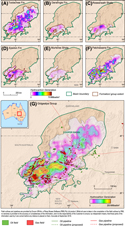 Figure 7. Hydrocarbon generation maps: (A) Toolachee Formation (Fm), (B) Daralingie Fm, (C) Roseneath Shale, (D) Epsilon Fm, (E) Murteree Shale, (F) Patchawarra Fm, and (G) all Gidgealpa Group. MMboe = million BOE; NSW = New South Wales; NT = Northern Territory; QLD = Queensland; SA = South Australia; TAS = Tasmania; WA = Western Australia.
The TOC content and HIo are also important factors in determining the relative hydrocarbon volumes expelled by each source rock. The contribution to total volumes generated by source facies type is fairly even, because the inherently high TOC content of the coal intervals (TOC > 50 wt. %) compensates for the greater thickness of the shales (TOC 0.5–50 wt. %). Although all source rocks can be modeled using a Pepper and Corvi (1995a) D/E/F organofacies, Hall et al. (2016a) noted a difference in HIo between the shales (TOC < 10 wt. %; HIo ∼140–160 mg HC/g TOC) and those with a higher contribution of coal (TOC > 10 wt. %; HIo ∼205–245 mg HC/g TOC). This higher HIo increases the volume of hydrocarbons expelled from coals compared with shales in the model.
Maximum paleotemperature has a smaller influence on the total hydrocarbons generated than the source-rock amount and quality. Within the Toolachee Formation, greater maximum burial depths in the Nappamerri and Windorah troughs result in higher TRs and generated volumes compared with the less mature basin margins. In contrast, the majority of the Patchawarra Formation has reached sufficient temperatures for generation to occur across all depocenters, with the exception of the Weena trough.
Although hydrocarbon generation began in the Permian in the deeper formations of the Nappamerri trough, the majority of generation occurred in the middle Cretaceous, coincident with the maximum depth of burial. This is consistent with the work of Deighton et al. (2003) but contrasts to earlier studies (Kantsler et al., 1986; Pitt, 1986) that proposed that generation commenced in the Late Cretaceous to Paleogene.
Fluid Composition
Hydrocarbons Expelled
The total liquid and total gas expelled from the Permian source rocks of the Cooper Basin are estimated to be 512 billion bbl (81 TL) and 4410 tcf (125 Tm3), respectively, with the largest contributions coming from the Toolachee and Patchawarra Formations (Figure 8; Table 6).
 Figure 8. Toolachee Formation coal source rock: (A) gas expelled, (B) liquid expelled, (C) gas retained, and (D) liquid retained. Toolachee Formation shale–coaly shale source rock: (E) gas expelled, (F) liquid expelled, (G) gas retained, and (H) liquid retained. Patchawarra Formation coal source rock: (I) gas expelled, (J) liquid expelled, (K) gas retained, and (L) liquid retained. Patchawarra Formation shale–coaly shale source rock: (M) gas expelled, (N) liquid expelled, (O) gas retained, and (P) liquid retained. NSW = New South Wales; QLD = Queensland; SA = South Australia.
Although the results from this study are not directly comparable with those from Deighton et al. (2003), because different source rocks were included in the model, the modeled volumes are of a similar order of magnitude. The GLR of fluids expelled from each source rock ranges from approximately 7000 to greater than 20,000 scf/bbl (∼1246‒3560 m3/m3; Table 6). The predicted hydrocarbon type is therefore gas condensate, with some light oil in areas of lower thermal maturity. This result is consistent with the observed dominance of gas condensate in the basin overall, with oil accumulations mostly being present in shallower reservoirs exposed to leakage and gas removal by water washing (see Discussion section below for further details).
Maximum liquids generation is achieved for the best-case (10% exceedence probability) HIo scenario for the coals of the Patchawarra Formation (Table 4). This gives an expelled fluid GLR of approximately 2000–9000 scf/bbl (∼356‒1600 m3/m3), suggesting that the expelled products will primarily be gas condensates, with light oil below Ro approximately 1.1% (TR < 50 wt. %). The lower HIo values in the shales, especially in the Roseneath and Murteree Shales, result in GLRs of 8000–50,000 scf/bbl (1423‒8897 m3/m3), which indicate that the expelled products will mainly be gas condensates.
The modeled GLR values are consistent with both the estimated system GLR calculated from the total identified resources (18,900 scf/bbl [3363 m3/m3]) and the observed system GLR values for the Patchawarra trough (12,000–30,000 scf/bbl [2135‒5338 m3/m3]) calculated from production test data (Department of State Development South Australia, 2017). The total production GLR for the basin is higher at approximately 67,000 scf/bbl (∼11,933 m3/m3). Although the system GLR calculated from production tests may be biased based on what has been economical to produce, an additional major contributing factor to this difference is the effect of secondary in-reservoir cracking, which is not included in the above model results. Cracking becomes significant at temperatures greater than 165°C, rapidly increasing GLR as oil cracks to gas. Thermal modeling shows that the temperatures at the base of the Cooper Basin section are less than 165°C across most of the Patchawarra trough (Hall et al., 2016c). As a result, the effects of cracking are likely to be minimal in this region, and comparison of the Patchawarra trough system GLR numbers with the modeled GLRs is appropriate. In contrast, thermal modeling shows that temperatures in the Nappamerri trough range from greater than 200°C at the base of the Cooper Basin section to 160°C at the top Toolachee Formation (Hall et al., 2016c). Secondary cracking would have therefore influenced almost all fluids reservoired within the Permian section, resulting in much higher GLRs and increasing the basin-wide average.
Although there is significant uncertainty surrounding the modeled GLR result, the full conversion expulsion GLR of approximately 12,000 scf/bbl (∼2135 m3/m3) is broadly consistent with a dew point fluid system, in which gas condensate is the primary expelled and migrating fluid and in which oil rims form where these fluids move into shallower reservoirs where the PVT conditions are below the fluid’s dew point.
Hydrocarbons Retained
The total liquid retained is estimated at 362 billion bbl (58 TL), and the total gas retained is estimated at 3568 tcf (101 Tm3; Figure 8; Table 6). The majority of both liquids and gas retained are in the Toolachee and Patchawarra Formations rather than either the Daralingie and Epsilon Formations or the Roseneath and Murteree Shales. The retained liquid and gas are split fairly evenly between lithologies, with 1653 tcf (47 Tm3) of gas (46% of the total gas) and 189 billion bbl (31 TL) of liquids (52% of the total liquids) retained within the coals. The broad spatial distribution of hydrocarbons remaining within the source rocks, especially those within the Toolachee and Patchawarra Formations, suggests the potential for widespread shale and deep dry coal plays. Furthermore, the volume of hydrocarbons retained within the source rocks of the Toolachee and Patchawarra Formations far exceeds the volumes of hydrocarbons retained within the Roseneath and Murteree Shales.
Uncertainty Analysis
Monte Carlo simulations were used to investigate the impact of input data uncertainty on the model results and to highlight any key dependencies that may exist between the input parameters.
The starting point for the Monte Carlo simulations was the deterministic basin model representing the best understanding of the basin’s evolution described in the previous sections. Uncertainty distributions were assigned to each input parameter, including fetch area, source depth, source thickness, thermal gradient, TOC content, HI, and kerogen kinetics. For each input parameter, an appropriate probability distribution was defined based on observed data distributions and underlying model assumptions, as discussed in the previous sections. The primary focus of this step was to capture the uncertainty in total hydrocarbon generation; hence, neither expulsion parameters nor oil and gas migration losses were considered here. In addition, there is considerable, fundamental uncertainty in the expulsion and retention behavior of different source-rock units and lithologies; however, investigation of this aspect is beyond the scope of the present study. The chosen distributions and ranges for each parameter are summarized in Table 7.

The Monte Carlo simulation randomly sampled the uncertainty space 3000 times, and results were aggregated to build the total-hydrocarbons-generated probability distributions for each source-rock unit. The results are expressed as exceedance probabilities, representing the chance or probability that the resource amount is greater than or equal to that value (where P10, P50, and P90 represent 10%, 50%, and 90% exceedance probabilities, respectively).
The total modeled volume of hydrocarbons generated from the Permian source rocks of the Cooper Basin is estimated to be approximately 1750 billion BOE (∼278 TL equivalent; P50 scenario); however, the difference between the P90 (∼730 billion BOE [∼116 TL equivalent]) and P10 (∼4100 billion BOE [∼652 TL equivalent]) scenarios highlights the range of uncertainties inherent in the modeling (Figure 9; Table 8). The P50 scenario is lower than the deterministic case (Table 8), reflecting the effects of the skewed input probability distribution functions, including the log-normal TOC distributions.
 Figure 9. Maximum theoretical hydrocarbon yield by source rock with uncertainties. Bboe = billion BOE; Fm = Formation; P10 = 10% exceedance probability; P50 = 50% exceedance probability; P90 = 90% exceedance probability.

The sensitivity of total generated hydrocarbon volumes to each of the input parameters and their ranking order are shown on the tornado diagrams in Figure 10 for the Patchawarra Formation coals and shale–coaly shale source rocks. For the shale–coaly shale intervals, TOC content has the biggest impact on uncertainty, resulting from the mixed lithologies contained within these source rocks. To reduce the uncertainty, shales (TOC < 10 wt. %) and coaly shales (TOC 10‒50 wt. %) would need to be modeled separately; however, the resolution of the regional electrofacies analyses is not good enough to distinguish the relative thicknesses of these. More detailed log analysis of a few key wells may be sufficient to break out the proportion of the net shale versus coaly shale facies. For coals (TOC > 50 wt. %), the variation in original HI has the biggest impact on uncertainty. Because the TOC range for clean coals is relatively more restricted, the sensitivity of total hydrocarbons generated to this parameter is lower.
 Figure 10. Tornado diagrams comparing the relative impact of each input parameter for (A) Patchawarra Formation shales–coaly shales and (B) Patchawarra Formation coals. Bboe = billion BOE; HI = hydrogen index; P10 = 10% exceedance probability; P50 = 50% exceedance probability; P90 = 90% exceedance probability; TOC = total organic carbon.
DISCUSSION
Comparison with Global Basins
The relationship between the total volume of hydrocarbons generated and that estimated to be in place has been used by previous studies to investigate the relative efficiency in which generated hydrocarbons are retained within conventional accumulations in a basin (e.g., Magoon and Valin, 1994; Biteau et al., 2010). Based on a compilation of more than 170 globally distributed basins, Biteau et al. (2010) estimated that the percentage of hydrocarbons retained in conventional accumulations represented between 0.1% and 50% of the total volumes generated. The most efficient basins, those with the highest percentage of hydrocarbons retained within accumulation, are compact, with close proximity between source, reservoir, and seal. In contrast, the least efficient systems are observed in Paleozoic and Proterozoic basins where complex structural histories commonly lead to phase changes and trap breaching.
As of December 2014, the total identified resources (remaining identified and produced) in the Cooper and Eromanga Basins included 447 million bbl (71 GL) of oil, 160 million bbl (25 GL) of condensate, 220 million bbl (35 GL) of liquefied petroleum gas, and 10.2 tcf (289 Gm3) of gas (Australian Energy Resources Assessment, 2017). A further 82 million bbl (13 GL) of oil and 0.9 tcf (25 Gm3) of gas of undiscovered conventional resources are also estimated to be present (Australian Energy Resources Assessment, 2017). The total conventional resources (discovered and undiscovered) represent 0.12% of the total modeled hydrocarbons generated. This falls at the lower end of the range published by Biteau et al. (2010), indicating that the system is lower efficiency. This is a consequence of the high charge volumes caused by thick coal sequences and average high thermal gradient on the supply side being offset by large losses from conventional plays because of the lack of continuous marine shale seals, early charge, and water washing. It should be noted that an excess of charge does not bear directly on the probability of underfill at the trap level (Bishop, 2015). However, a large charge excess increases the probability of long-distance migration, helps to overcome losses resulting from all causes, and allows pervasive permeation of the migration network. All of these factors should lead to high exploration success rates overall.
The disparity between the predicted volume of hydrocarbons expelled and the volume estimated to be captured in conventional reservoirs highlights the potential for large volumes to remain within unconventional plays, both retained within and near the source rocks, and within lower-porosity (tight) reservoirs. For a further three basins, Biteau et al. (2010) estimated that the percentage of hydrocarbons retained in unconventional accumulations represented more than 50% of the total volumes generated. The best-estimate (P50) shale gas and liquids in place for the Murteree and Roseneath Shales are 43.6 tcf (1.2 Tm3) and 4.5 billion bbl (0.7 TL) and 93.1 tcf (2.6 Tm3) and 4.2 billion bbl (0.7 TL), respectively (Australian Energy Resources Assessment, 2017). The best-estimate (P50) total tight gas- and liquids-in-place resources of the Patchawarra, Epsilon, Daralingie, and Toolachee Formations are an order of magnitude larger, at 1019 tcf (29 Tm3; including dry, wet, and associated gas) and 490 billion bbl liquids (78 TL; including oil and gas condensate; Geoscience Australia, 2017a). This gives a total estimated in-place resource for both conventional and unconventional accumulations of 700 billion BOE (115 TL equivalent), approximately 30% of the total hydrocarbons generated.
To date, no basin-wide, undiscovered resource estimates have been published for the Patchawarra, Epsilon, Daralingie, and Toolachee deep coal and shale plays. However, once undiscovered resources are available for all play types, the total estimated in-place resources are likely to rise to greater than 50%, consistent with the unconventional basins evaluated by Biteau et al. (2010). The remaining difference between the total volume of generated hydrocarbons and an undiscovered resources estimate including all plays would provide an indication of the total hydrocarbon loss from the system.
Type of Discovered Fluids as a Constraint on Volumes Generated and Retained
The main uncertainties in the modeled generated hydrocarbons are the average TOC values assigned to the shale‒coaly shale source rocks and the HIo assigned to the coals. Uncertainty also exists for the generated and retained hydrocarbon proportions, arising from uncertainty in the input parameters to the ARCO expulsion model. The range is not large, however, at approximately 13%–45% retention of the total generated gas for a wide range of values for initial oil sorption, inorganic porosity, maximum inorganic saturation, and organic porosity reduction factor. Hence, uncertainty in the generated volume is more relevant than in expelled versus retained amounts, and the largest impact on this is the HIo of the coals.
Because source-rock HIo is the strongest determinant of the GLR of the expelled fluids, appropriate HIo values should also predict field GLRs that are consistent with observations. The base-case source-rock characteristics result in expelled fluid GLRs ranging from 2700 scf/bbl (480 m3/m3) at TR = 20% to 6400 scf/bbl (1139 m3/m3) at TR = 50% to 33,000 scf/bbl (5872 m3/m3) at TR = 90% (equivalent to a maturity > 1.9% Ro). Typically, fluids with a GLR of less than approximately 3000 scf/bbl (∼534 m3/m3) will result in either single-phase oil or oils with a gas cap. Fluids with GLRs greater than approximately 5000 scf/bbl (∼890 m3/m3) will result in either mainly gas-condensate accumulations or gas with oil rims. Hence, although it is expected that some light oil with gas caps would be present in reservoirs draining low-maturity Permian coals, the dominant expelled fluid type is predicted to be a gas condensate with GLR in the range of approximately 5000–50,000 scf/bbl (∼89–8897 m3/m3). This corresponds to condensate–gas ratios (CGRs) between 20 and 200 bbl/million scf. However, the high end of this range may not be seen, because in most reservoirs such fluids will be below their saturation pressure (dew point), and liquids will have dropped out as an oil rim.
Before comparing the model predictions with the observed fluid types and GLRs, two factors need to be considered that could confound the comparison: (1) alteration of GLR in the reservoir or during migration and (2) the possibility that other source rocks contribute.
Impact of Water Washing
Considering in-reservoir alteration first, most Cooper–Eromanga fluids are not significantly biodegraded, but there is strong evidence that oils in the Eromanga Basin reservoirs are water washed (Cotton and McKirdy, 2006 and references therein; Elliott, 2015b). In addition, Permian fluids within the deep coal reservoirs may also have experienced diffusive gas loss where adjacent to overlying aquifers of the Great Artesian Basin (Dunlop et al., 1992, 2017).
Depletion in light aromatics such as toluene relative to alkanes is the most commonly cited indicator for water washing (Lafargue and Le Thiez, 1996; de Hemptinne et al., 2001). However, methane is among the most water-soluble hydrocarbons and is more soluble than light aromatics (such as benzene and toluene) at elevated pressures (Price, 1979; Duan et al., 1992). Hence, water washing selectively removes methane and can reduce GLR to the point where a gas condensate is converted to undersaturated oil (Newell, 1999).
In cases where water washing is responsible for reduced GLR, this should be apparent in a reduction in the amount of methane relative to ethane, propane, and other straight-chain hydrocarbons, that is, an increase in gas “wetness.” Figure 11A shows a comparison of GLR with gas wetness (sum of mole percent ethane to pentane divided by the total of methane though to pentane) for a set of Cooper–Eromanga fluids. These fluids have been selected because they have complete and internally consistent molecular compositional data available in their PVT reports. Figure 11B shows a comparison of saturation pressure with reservoir pressure; note that the data set is smaller here because saturation pressures are not reported for all points.
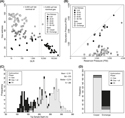 Figure 11. Bulk fluid composition from Cooper and Eromanga reservoirs. (A) Gas–liquid ratio (GLR) versus gas wetness. (B) Reservoir pressure versus saturation pressure. (C) Histogram of bulk fluid composition by reservoir depth. (D) Histogram of bulk fluid composition by basin. N = number of samples; Std = standard deviation.
Figure 11A, B shows that (1) there is much more scatter in the gas wetness values for the Eromanga Basin compared with the Cooper Basin reservoired fluids, (2) the majority of the Eromanga Basin fluids are highly gas-undersaturated oils, and (3) the solution gases of these oils are very “wet.” These observations are consistent with variable but generally high gas loss from the Eromanga Basin reservoir fluids resulting from water washing. Before this process occurred, it is likely that the original fluids were gas condensates or gas-rich oils. This is also consistent with the high API gravity of the Eromanga Basin oils (median 47°).
Contribution from Non-Permian Source Rocks
The contribution of non-Permian source rocks to the fluids observed has also been considered. Excellent potential source rocks exist within the Eromanga Basin strata, particularly in the Middle Jurassic succession (Michaelsen and McKirdy, 1996 and references therein). However, these are thermally immature or marginally mature in most parts of the basin. On this basis alone, the contribution from the intra-Eromanga source rocks should be minor, except in a few localized areas. Despite this, several reports argue for a more significant contribution, and most recently Plummer (2016, p. 43) stated that “a number of oils were either derived solely from or had a significant input from, mature Jurassic source rocks.” Various kinds of geochemical data underpin this conclusion, and the interpretations are robust in themselves. However, they do not sufficiently consider the quantitative aspects of fluid mixing. Arouri and McKirdy (2005) have shown that some biomarker features commonly used to define the Jurassic versus Permian contribution seriously overestimate the Jurassic contribution. This conclusion applies to the origin of the liquid component of the whole fluids, but we must also consider what happens when a Permian-derived gas condensate either mixes with a small amount of Jurassic oil or comes into contact with early mature and organically rich Jurassic source rocks. A gas condensate with a GLR of 20,000 scf/bbl (3559 m3/m3; CGR 50 bbl/million scf) has a gas to liquids mass ratio of approximately 4:1, whereas this ratio is approximately 1:10 for an oil from a low-maturity source rock. This means that a whole fluid derived from Permian and Jurassic source rocks in a mass proportion of 40:1 will have approximately equal contributions to the liquids fraction from each source. Since virtually all geochemical source assignments for fluids from the Cooper and Eromanga Basins have been based on analysis of the liquids fraction alone, it is inevitable that the Jurassic source contribution would be overestimated. This problem is exacerbated by the postemplacement loss of gas by water washing, as described above for Eromanga Basin reservoirs.
An original charge of Cooper Basin Permian gas condensate, followed by gas loss in Eromanga Basin reservoirs, has resulted in an unusually distinct separation of gas and oil pools both by depth and between the Cooper and Eromanga Basins. This is shown for a basin-wide data set of fluids in Figure 11C, D. The spatial distribution of these data confirms the occurrence of oil mainly close to the zero edge of the Cooper Basin and on intrabasin highs where Permian-sourced fluids can enter the Eromanga Basin reservoirs and be exposed to gas loss by water washing (Figure 12).
 Figure 12. (A) Spatial distribution of reservoir fluids colored by bulk composition. (B) Cross section showing reservoir fluid variation with depth. equiv. = equivalent; Fm = Formation; Gp = Group; NSW = New South Wales; NT = Northern Territory; QLD = Queensland; SA = South Australia; Sh. = Shale; Ss = Sandstone; TAS = Tasmania; VIC = Victoria; WA = Western Australia.
The less altered Cooper Basin reservoir fluids thus provide the best comparison between the GLRs observed and those predicted by the charge model. The GLRs for these fluids range from 2000 to greater than 200,000 scf/bbl (356–35,587 m3/m3), but most lie between 10,000 and 100,000 scf/bbl (1779–17,794 m3/m3; corresponding to gas condensates with CGRs of 10 to 100 bbl/million scf). These GLRs are approximately double those predicted by the model (5000 to 50,000 scf/bbl [890–8897 m3/m3]). This may seem like a large discrepancy, but relatively small changes in HIo and in the kinetics of cracking of the retained oil are enough to cause differences of this magnitude. In addition, secondary in-reservoir cracking of expelled liquids within the Nappamerri trough will further impact this. Overall, the agreement of the model prediction with the observed fluid type and distribution is considered satisfactory.
CONCLUSIONS
This study used PSA to provide a regional framework for understanding both the conventional and unconventional hydrocarbon prospectivity of the Cooper Basin, Australia. Results have quantified the spatial distribution and petroleum generation potential of Permian source rocks across the basin as well as the likely composition of both expelled and retained fluids. The deterministic petroleum systems model estimated the volumes of expelled and retained hydrocarbons at 512 billion bbl (84 TL) and 4410 tcf (125 Tm3) and 362 billion bbl (58 TL) and 3568 tcf (101 Tm3), respectively. The combined theoretical volume of hydrocarbons generated from all Permian source rocks is mapped, highlighting the broad extent of the source kitchens and its consistency with the location of major conventional fields across the basin. Source rocks within the Toolachee and Patchawarra Formations are the biggest contributors to both expelled and retained hydrocarbons, because these are the richest, thickest, and most extensive source facies, with good to excellent generation potential across the entire basin. In contrast, the hydrocarbon volumes generated from the Roseneath and Murteree Shales are an order of magnitude less, because the shale facies are volumetrically smaller and their source rocks are of lower quality.
The modeled GLR of expelled fluids from each source rock ranges between approximately 7000 and 22,000 scf/bbl (∼1246‒3915 m3/m3). When secondary in-reservoir cracking is considered, this is broadly consistent with the production GLR to date of 67,000 scf/bbl (11,922 m3/m3). Small, but nevertheless significant, commercial pools of undersaturated oil occur primarily in Eromanga Basin reservoirs, although some are also present in the Cooper Basin. These are mostly the remnant liquids from Permian-sourced gas condensates with a subsidiary contribution from Jurassic source rocks in localized areas where these are mature.
Monte Carlo simulations were used to quantify the uncertainty associated with hydrocarbon yield and investigate the sensitivity of results to each input parameter. The difference between the P90 (∼730 billion BOE [∼116 TL equivalent]) and P10 (∼4100 billion BOE [∼652 TL equivalent]) scenarios highlights the large inherent uncertainty. For the shale‒coaly shale source rocks, the biggest contribution to this uncertainty comes from the broad distribution of TOC values (0.5‒50 wt. %). In contrast, for the coal source rocks (TOC > 50 wt. %), variation in HIo contributes most.
The large total generation potential of the Cooper Basin and the broad distribution of the Permian source kitchen highlight the basin’s significance as a hydrocarbon province. The large disparity between the calculated volumes of hydrocarbons generated and the volumes found in reservoirs indicates the potential for large volumes to remain within the basin, despite significant losses from leakage and water washing. The hydrocarbons expelled have provided abundant charge to both conventional accumulations and to lower-porosity (tight) reservoirs, and the broad spatial distribution of hydrocarbons remaining within the source rocks, especially those within the Toolachee and Patchawarra Formations, suggests the potential for widespread shale and deep dry coal plays.
The results presented here provide a starting point for hydrocarbon migration and accumulation analyses, which would provide insights into fluid movement through the basin and help to understand the effects processes such as phase separation, migration losses, and seal integrity have on the resultant fluid compositions. This model also has the potential to be extended to include maturity, generation, migration, and accumulation modeling in the overlying Eromanga Basin. Further consideration also needs to be given to the source potential of the underlying basins, including the Devonian sediments of the Warrabin trough and Barrolka depression in the north and the Cambrian–Ordovician Warburton Basin in the south, to support geochemical evidence for oil migration into the overlying Cooper Basin sediments (Boreham and Summons, 1999).
REFERENCES CITED
Alexander, E. M., D. I. Gravestock, C. Cubitt, and A. Chaney, 1998, Chapter 6: Lithostratigraphy and environments of deposition, in D. I. Gravestock, J. E. Hibburt, and J. F. Drexel, eds., The petroleum geology of South Australia: Cooper Basin: Adelaide, Australia, South Australia Department of Primary Industries and Resources, v. 4, p. 69–115.
Alexander, E. M., A. Sansome, and T. B. Cotton, 2006, Chapter 5: Lithostratigraphy and environments of deposition, in T. B. Cotton, M. F. Scardigno, and J. E. Hibburt, eds., The petroleum geology of South Australia, 2nd ed.: Eromanga Basin: Adelaide, Australia, South Australia Department of Primary Industries and Resources, v. 2, 129 p.
Allen, A. A., and J. R. Allen, 2005, Basin analysis: Principles and applications, 2nd ed.: Malden, Massachusetts, Blackwell, 549 p.
Arouri, K. R., and D. M. McKirdy, 2005, The behaviour of aromatic hydrocarbons in artificial mixtures of Permian and Jurassic end-member oils: Application to in-reservoir mixing in the Eromanga Basin, Australia: Organic Geochemistry, v. 36, no. 1, p. 105–115, doi:10.1016/j.orggeochem.2004.06.015.
Beach Energy, 2011a, Encounter 1 well completion report, PEL 218, Adelaide, Australia, 868 p., accessed April 25, 2017, https://sarigbasis.pir.sa.gov.au/WebtopEw/ws/samref/sarig1/image/DDD/ENCOUNTER%20001.zip.
Beach Energy, 2011b, Holdfast 1 well completion report, PEL 218, Adelaide, Australia, 1236 p., accessed April 25, 2017, https://sarigbasis.pir.sa.gov.au/WebtopEw/ws/samref/sarig1/image/DDD/HOLDFAST%20001.zip.
Beardsmore, G. R., 2004, The influence of basement on surface heat flow in the Cooper Basin: Exploration Geophysics, v. 35, no. 4, p. 223–235, doi:10.1071/EG04223.
Beardsmore, G. R., and J. P. Cull, 2001, Crustal heat flow: A guide to measurement and modelling: Cambridge, United Kingdom, Cambridge University Press, 324 p., doi:10.1017/CBO9780511606021.
Bishop, R. S., 2015, Implications of source overcharge for prospect assessment: Interpretation, v. 3, no. 2, p. T93–T107, doi:10.1190/INT-2014-0114.1.
Biteau, J. J., J. C. Heidmann, G. Choppin de Janvry, and B. Chevallier, 2010, The whys and wherefores of the SPI–PSY method for calculating the world hydrocarbon yet-to-find figures: First Break, v. 28, no. 11, p. 53–64.
Boreham, C. J., 2013, Rock-Eval pyrolysis data of selected samples from wells drilled in the Cooper Basin, South Australia, Australia: Canberra, Australia, Geoscience Australia Destructive Analysis Report 1432, 20 p.
Boreham, C. J., and A. J. Hill, 1998, Chapter 8: Source rock distribution and hydrocarbon geochemistry, in D. I. Gravestock, J. E. Hibburt, and J. F. Drexel, eds., The petroleum geology of South Australia: Cooper Basin: Adelaide, Australia, South Australia Department of Primary Industries and Resources, v. 4, p. 131–144.
Boreham, C. J., B. Horsfield, and H. J. Schenk, 1999, Predicting the quantities of oil and gas generated from Australian Permian coals, Bowen Basin using pyrolytic methods: Marine and Petroleum Geology, v. 16, no. 2, p. 165–188, doi:10.1016/S0264-8172(98)00065-8.
Boreham, C. J., and R. E. Summons, 1999, New insights into the active petroleum systems in the Cooper and Eromanga basins, Australia: Australian Petroleum Production and Exploration Association Journal, v. 39, no. 1, p. 263–296, doi:10.1071/AJ98016.
Bureau of Meteorology, 2015, Mean monthly and mean annual temperature data, accessed March 3, 2015, http://www.bom.gov.au/jsp/ncc/climate_averages/temperature/index.jsp.
Burnham, A. K., and J. J. Sweeney, 1989, A chemical kinetic model of vitrinite maturation and reflectance: Geochimica et Cosmochimica Acta, v. 53, no. 10, p. 2649–2657, doi:10.1016/0016-7037(89)90136-1.
Carr, L. K., R. J. Korsch, T. J. Palu, and B. Reese, 2016, Onshore basin inventory: The McArthur, South Nicholson, Georgina, Wiso, Amadeus, Warburton, Cooper and Galilee basins, central Australia: Geoscience Australia Record 2016/04, 174 p.
Channon, G. J., and G. R. Wood, 1989, Stratigraphy and hydrocarbon prospectivity of Triassic sediments in the northern Cooper Basin, South Australia: Adelaide, Australia, Department of Mines and Energy Confidential Envelope 8126, 50 p.
Cook, A. G., S. E. Bryan, and J. J. Draper, 2013, Chapter 7: Post-orogenic Mesozoic basins and magmatism, in Jell, P. A., ed., Geology of Queensland: Brisbane, Australia, Geological Survey of Queensland, p. 515–575.
Cook, A. G., and P. A. Jell, 2013, Chapter 8: Paleogene and Neogene, in P. A. Jell, ed., Geology of Queensland: Brisbane, Australia, Geological Survey of Queensland, p. 577–652.
Cook, A. C., and N. R. Sherwood, 1991, Classification of oil shales, coals and other organic-rich rocks: Organic Chemistry, v. 17, p. 211–222.
Cotton, T. B., and D. M. McKirdy, 2006, Chapter 10: Hydrocarbon generation and migration, in T. B. Cotton, M. F. Scardigno, and J. E. Hibburt, eds., The petroleum geology of South Australia, 2nd ed.: Eromanga Basin: Adelaide, Australia, South Australia Department of Primary Industries and Resources, v. 2, 22 p.
Dahl, J. E., J. M. Moldowan, K. E. Peters, G. E. Claypool, M. A. Rooney, G. E. Michael, M. R. Mellow, and M. L. Kohnen, 1999, Diamondoid hydrocarbons as indicators of natural oil cracking: Nature, v. 399, no. 6731, p. 54–57, doi:10.1038/19953.
de Hemptinne, J.-C., R. Peumery, V. Ruffier-Meray, G. Moracchini, J. Naiglin, B. Carpentier, J. L. Oudin, and J. Connan, 2001, Compositional changes resulting from the water-washing of a petroleum fluid: Journal of Petroleum Science Engineering, v. 29, no. 1, p. 39–51, doi:10.1016/S0920-4105(00)00089-9.
Deighton, I., J. J. Draper, A. J. Hill, and C. J. Boreham, 2003, A hydrocarbon generation model for the Cooper and Eromanga Basins: Australian Petroleum Production and Exploration Association Journal, v. 43, no. 1, p. 433–451, doi:10.1071/AJ02023.
Deighton, I., and A. J. Hill, 1998, Chapter 9: Thermal and burial history, in D. I. Gravestock, J. E. Hibburt, and J. F. Drexel eds., The petroleum geology of South Australia: Cooper Basin: Adelaide, Australia, South Australia Department of Primary Industries and Resources, v. 4, p. 143–155.
Department for Manufacturing, Innovation, Trade, Resources and Energy, 2001, Seismic mapping data sets over the Cooper Basin sector, South Australia 2001, accessed April 25, 2017, https://sarig.pir.sa.gov.au/Map.
Department for Manufacturing, Innovation, Trade, Resources and Energy, 2009, Seismic mapping data sets over the Cooper Basin sector, South Australia 2009, accessed April 25, 2017, https://sarig.pir.sa.gov.au/Map.
Department of Natural Resources and Mines Queensland Government, 2017, Queensland petroleum exploration data (QPED), accessed April 25, 2017, https://data.gov.au/dataset/cb357721-bf22-45c9-a82e-828807912dd4.
Department of State Development South Australia, 2017, PEPS-SA (petroleum and geothermal attribute database), accessed April 25, 2017, http://petroleum.statedevelopment.sa.gov.au/data_and_publications/peps-sa.
Draper, J. J., ed., 2002, Geology of the Cooper and Eromanga Basins: Brisbane, Australia, Queensland Department of Natural Resources and Mines, 85 p.
Draper, J. J., C. J. Boreham, K. L. Hoffmann, and J. L. McKellar, 2004, Devonian petroleum systems in Queensland, in P. J. Boult, D. R. Johns, and S. C. Lang, eds., PESA’s Eastern Australasian Basins Symposium II conference proceedings: Petroleum Exploration Society of Australia Eastern Australasian Basins Symposium II, Adelaide, Australia, September 19–22, 2004, p. 297–318.
Duan, Z., N. Møller, J. Greenberg, and J. H. Weare, 1992, The prediction of methane solubility in natural waters to high ionic strength from 0 to 250°C and from 0 to 1600 Bar: Geochimica et Cosmochimica Acta, v. 56, no. 4, p. 1451–1460, doi:10.1016/0016-7037(92)90215-5.
Duddy, I. R., and M. E. Moore, 1999, Thermal history reconstruction in Cooper-Eromanga Basin wells using apatite and zircon fission track analysis and vitrinite reflectance: Adelaide, Australia, Geotrack Report 668: Primary Industries and Resources South Australia Open File Envelope 8426, 229 p.
Dunlop, E. C., M. V. Browne, and E. F. Tadiar, 1992, Depletion of gas reservoirs by molecular diffusion—A case study: Australian Petroleum Exploration Association Journal, v. 32, p. 369–390.
Dunlop, E. C., D. S. Warner, P. E. R. Warner, and L. R. Coleshill, 2017, Ultra-deep Permian coal gas reservoirs of the Cooper Basin: Insights from new studies: Australian Petroleum Production and Exploration Association Journal, v. 57, no. 1, p. 218–262, doi:10.1071/AJ16015.
Elliott, L. G., 2015a, Using biodegradation to date hydrocarbon entry into reservoirs: Examples from the Cooper/Eromanga Basin, Australia: AAPG Search and Discovery article 41749, accessed April 25, 2017, http://www.searchanddiscovery.com/documents/2015/41749eliott/ndx_elliott.pdf.
Elliott, L. G., 2015b, Water-washing: A major hydrocarbon alteration process. Part 2—Processes, controls and hydrocarbon type prediction: AAPG Search and Discovery article 41750, accessed April 25, 2017, http://www.searchanddiscovery.com/documents/2015/41750elliott/ndx_elliott.pdf.
Eslinger, E., and R. V. Everett, 2012, Petrophysics in gas shales, in J. A. Breyer, ed., Shale reservoirs—Giant resources for the 21st century: AAPG Memoir 97, p. 419–451.
Gallagher, K. L., 1988, The subsidence history and thermal state of the Eromanga and Cooper Basins, Ph.D. thesis, Australian National University, Canberra, Australia, 407 p.
Geoscience Australia, 2017a, Australian energy resources assessment, accessed March 6, 2017, http://aera.ga.gov.au/.
Geoscience Australia, 2017b, National petroleum wells database, accessed April 25, 2017, http://dbforms.ga.gov.au/www/npm.well.search.
Geoscience Australia, 2017c, Stratigraphic names database, accessed April 25, 2017, http://www.ga.gov.au/data-pubs/data-standards/reference-databases/stratigraphic-units.
Goldstein, B., S. Menpes, A. Hill, A. Wickham, E. Alexander, M. Jarosz, and D. Pepicelli, et al, 2012, Roadmap for unconventional gas projects in South Australia: Adelaide, Australia, Department for Manufacturing, Innovation, Trade, Resources and Energy, Energy Resources Division, 258 p.
Gravestock, D. I., J. E. Hibburt, and J. F. Drexel, eds., 1998, Petroleum geology of South Australia: Cooper Basin: Adelaide, Australia, South Australia Department of Industries and Resources, v. 4, 236 p.
Gray, A. R. G., and J. J. Draper, 2002, Petroleum geology, in Draper, J. J., ed., Geology of the Cooper and Eromanga Basins: Brisbane, Australia, Queensland Department of Natural Resources and Mines, p. 63–74.
Gray, A. R. G., and J. L. McKellar, 2002, Cooper Basin stratigraphy, in Draper, J. J., ed., Geology of the Cooper and Eromanga Basins: Brisbane, Australia, Queensland Department of Natural Resources and Mines, p. 9–26.
Gray, A. R. G., M. McKillop, and J. L. McKellar, 2002, Eromanga Basin stratigraphy, in Draper, J. J., ed., Geology of the Cooper and Eromanga Basins: Brisbane, Australia, Queensland Department of Natural Resources and Mines, p. 30–56.
Hall, L. S., C. J. Boreham, D. S. Edwards, T. J. Palu, T. Buckler, A. J. Hill, and A. Troup, 2016a, Cooper Basin source rock geochemistry: Regional hydrocarbon prospectivity of the Cooper Basin: Part 2: Canberra, Australia, Geoscience Australia Record 2016/06, 123 p., doi:10.11636/Record.2016.006.
Hall, L. S., A. J. Hill, A. Troup, R. Korsch, B. Radke, R. S. Nicoll, T. J. Palu, L. Wang, and A. Stacey, 2015, Cooper Basin architecture and lithofacies: Regional hydrocarbon prospectivity of the Cooper Basin: Part 1: Canberra, Australia, Geoscience Australia Record 2015/31, 97 p., doi:10.11636/Record.2015.031.
Hall, L. S., C. Lawson, D. S. Edwards, C. J. Boreham, T. J. Palu, A. J. Hill, and A. Troup, 2016b, Cooper Basin source rock atlas GIS: Canberra, Australia, Geoscience Australia accessed April 25, 2017, http://www.ga.gov.au/metadata-gateway/metadata/record/90687.
Hall, L. S., and T. J. Palu, 2016, Cooper Basin regional petroleum systems model, accessed April 25, 2017, http://www.ga.gov.au/metadata-gateway/metadata/record/100740.
Hall, L. S., T. J. Palu, A. P. Murray, C. J. Boreham, D. S. Edwards, A. J. Hill, and A. Troup, 2016c, Cooper Basin petroleum systems analysis: Regional hydrocarbon prospectivity of the Cooper Basin: Part 3: Canberra, Australia, Geoscience Australia Record 2016/29, 153 p., doi:10.11636/Record.2016.029.
Hantschel, T., and A. I. Kauerauf, 2009, Fundamentals of basin and petroleum systems modelling: Berlin, Springer-Verlag, 476 p., doi:10.1007/978-3-540-72318-9.
Holgate, F., and E. Gerner, 2010, Oz temp well temperature data: Canberra, Australia, Geoscience Australia, accessed April 25, 2017, https://data.gov.au/dataset/oztemp-well-temperature-data.
I’Anson, A., I. Deighton, R. D. Müller, A. Dutkiewicz, and C. Heine, 2018, Burial and exhumation history of the Galilee Basin, Australia: Implications for unconventional hydrocarbon prospectivity, AAPG Bulletin, v. 102, no. 3, p. 483–507, doi:10.1306/0608171609417067.
Jarvie, D. M., B. L. Claxton, F. Henk, and J. T. Breyer, 2001, Oil and shale gas from the Barnett Shale, Fort Worth Basin, Texas: AAPG National Convention, Denver, Colorado, June 3–6, 2001, 28 p.
Kantsler, A. J., T. J. Prudence, A. C. Cook, and M. Zwigulis, 1986, Hydrocarbon habitat of the Cooper/Eromanga Basin, Australia: Australian Petroleum Exploration Association Journal, v. 23, p. 75–92.
Kennett, B., M. Salmon, and E. Saygin, AusMoho Working Group, 2011, AusMoho: The variation of Moho depth in Australia: Geophysical Journal International, v. 187, no. 2, p. 946–958, doi:10.1111/j.1365-246X.2011.05194.x.
Korsch, R. J., and J. M. Totterdell, 2009, Subsidence history and basin phases of the Bowen, Gunnedah and Surat Basins, eastern Australia: Australian Journal of Earth Sciences, v. 56, p. 335–353, doi:10.1080/08120090802698687.
Korsch, R. J., J. M. Totterdell, T. Fomin, and M. G. Nicoll, 2009, Contractional structures and deformational events in the Bowen, Gunnedah and Surat Basins, eastern Australia: Australian Journal of Earth Sciences, v. 56, p. 477–499, doi:10.1080/08120090802698745.
Lafargue, E., and P. Le Thiez, 1996, Effect of water washing on light ends compositional heterogeneity: Organic Geochemistry, v. 24, no. 12, p. 1141–1150, doi:10.1016/S0146-6380(96)00095-2.
Magoon, L. B., and W. G. Dow, 1994, The petroleum system, in L. B. Magoon and W. G. Dow, eds., The petroleum system—From source to trap: AAPG Memoir 60, p. 3–24.
Magoon, L. B., and C. V. Valin, 1994, Overview of petroleum systems case studies, in L. B. Magoon and W. G. Dow, eds., The petroleum system—From source to trap: AAPG Memoir 60, p. 329–338.
Mahlstedt, N., R. di Primio, B. Horsfield, and C. J. Boreham, 2015, Multi-component kinetics and late gas potential of selected Cooper Basin source rocks: Canberra, Australia, Geoscience Australia Record 2015/19, 199 p., doi:10.11636/Record.2015.019.
Mavko, G., T. Mukerji, and J. Dvorkin, 2009, The rock physics handbook, tools for seismic analysis of porous media: Cambridge, United Kingdom, Cambridge University Press, 524 p., doi:10.1017/CBO9780511626753.
Mavromatidis, A., and R. R. Hillis, 2005, Quantification of exhumation in the Eromanga Basin and its implications for hydrocarbon exploration: Petroleum Geoscience, v. 11, no. 1, p. 79–92, doi:10.1144/1354-079304-621.
McKellar, J. L., 2013, The Cooper Basin, in P. A. Jell, ed., Geology of Queensland: Brisbane, Australia, Geological Survey of Queensland, p. 204–212.
Meixner, A. J., A. L. Kirkby, D. T. Lescinsky, and N. Horspool, 2012, The Cooper Basin 3D map version 2: Thermal modelling and temperature uncertainty: Canberra, Australia, Geoscience Australia Record 2012/60, 75 p.
Michaelsen, B. H., and D. M. McKirdy, 1996, Source rock distribution and hydrocarbon geochemistry, in E. M. Alexander and J. E. Hibburt, eds., The petroleum geology of South Australia: Eromanga Basin: Adelaide, Australia, South Australia Department of Mines and Energy, v. 2, p. 101–110.
Middleton, M. F., 1979, Heatflow in the Moomba, Big Lake and Toolachee gas fields of the Cooper Basin and implications for hydrocarbon maturation: Exploration Geophysics, v. 10, no. 2, p. 149–155, doi:10.1071/EG979149.
Middleton, A. W., I. T. Uysal, and S. D. Golding, 2015, Chemical and mineralogical characterisation of illite–smectite: Implications for episodic tectonism and associated fluid flow, central Australia: Geochimica et Cosmochimica Acta, v. 148, p. 284–303, doi:10.1016/j.gca.2014.09.035.
Moussavi-Harami, R., 1996, Burial history, in Alexander, E. M., and J. E. Hibburt, eds., Petroleum geology of South Australia: Eromanga Basin: Adelaide, Australia, South Australia Department of Mines and Energy, v. 2, p. 125–140.
National Geoscience Mapping Accord, 2001, NGMA Cooper and Eromanga Basins, Australia, seismic mapping data sets: Custodian—Department for Manufacturing, Innovation, Trade, Resources and Energy on behalf of the National Geoscience Mapping Accord, accessed April 25, 2017, https://sarig.pir.sa.gov.au/Map.
Newell, N. A., 1999, Water-washing in the Northern Bonaparte Basin: Australian Petroleum Production and Exploration Association Journal, v. 39, no. 1, p. 227–247, doi:10.1071/AJ98014.
Pasyanos, M. E., T. G. Masters, G. Laske, and Z. Ma, 2014, LITHO1.0: An updated crust and lithospheric model of the Earth: Journal of Geophysical Research, v. 119, p. 2153–2173.
Pepper, A. S., and P. J. Corvi, 1995a, Simple kinetic models of petroleum formation. Part I: Oil and gas generation from kerogen: Marine and Petroleum Geology, v. 12, no. 3, p. 291–319, doi:10.1016/0264-8172(95)98381-E.
Pepper, A. S., and P. J. Corvi, 1995b, Simple kinetic models of petroleum formation. Part III: Modelling an open system: Marine and Petroleum Geology, v. 12, no. 4, p. 417–452, doi:10.1016/0264-8172(95)96904-5.
Pepper, A. S., and P. J. Dodd, 1995, Simple kinetic models of petroleum formation. Part II: Oil-gas cracking: Marine and Petroleum Geology, v. 12, no. 3, p. 321–340, doi:10.1016/0264-8172(95)98382-F.
Peters, K. E., D. J. Curry, and M. Kacewicz, 2012, An overview of basin and petroleum system modeling: Definitions and concepts, in K. E. Peters, D. J. Curry, and M. Kacewicz, eds., Basin modeling: New horizons in research and applications: AAPG Hedberg Series 4, p. 1–16.
Peters, K. E., C. C. Walters, and J. M. Moldowan, 2005, The biomarker guide, volume 1, biomarkers and isotopes in the environment and human history: Cambridge, United Kingdom, Cambridge University Press, 429 p.
Pitt, G. M., 1986, Geothermal gradients, geothermal histories and the timing of thermal maturation in the Eromanga-Cooper Basins: Hornsby, Australia, Geological Society of Australia Special Publication 12, p. 323–351.
Plummer, P., 2016, Cooper/Eromanga Basin oil geochemistry: Evidence for multiple source intervals: Petroleum Exploration Society of Australia News, v. 143, p. 43–54.
Powell, T. G., C. J. Boreham, M. Smyth, N. Russell, and A. C. Cook, 1991, Petroleum source rock assessment in non-marine sequences: Pyrolysis and petrographic analysis of Australian coals and carbonaceous shales: Organic Geochemistry, v. 17, no. 3, p. 375–394, doi:10.1016/0146-6380(91)90101-O.
Price, L., 1979, Aqueous solubility of methane at elevated pressures and temperatures: AAPG Bulletin, v. 63, no. 9, p. 1527–1533.
Radke, B. M., J. R. Kellett, T. R. Ransley, and J. G. Bell, 2012, Lexicon of the lithostratigraphic and hydrogeological units of the Great Artesian Basin and its Cenozoic cover: A technical report to the Australian Government from the CSIRO Great Artesian Basin Water Resource Assessment: Canberra, Australia, Commonwealth Scientific and Industrial Research Organisation Water for a Healthy Country Flagship, 175 p.
Ransley, T. R., and B. D. Smerdon, eds., 2012, Hydrostratigraphy, hydrogeology and system conceptualisation of the Great Artesian Basin: A technical report to the Australian Government from the CSIRO Great Artesian Basin Water Resource Assessment: Canberra, Australia, Commonwealth Scientific and Industrial Research Organisation Water for a Healthy Country Flagship, 324 p.
Raza, A., K. Hill, and R. J. Korsch, 2009, Mid Cretaceous uplift and denudation of the Bowen and Surat basins, eastern Australia: Relationship to Tasman Sea rifting from apatite fission track and vitrinite reflectance data: Australian Journal of Earth Sciences, v. 56, no. 3, p. 501–531, doi:10.1080/08120090802698752.
Santos–Beach Energy–Origin Energy, 2012, Moomba 191 well completion report, South Australia, 1016 p., accessed April 25, 2017, https://sarigbasis.pir.sa.gov.au/WebtopEw/ws/samref/sarig1/image/DDD/MOOMBA%20191.zip.
Stewart, A. J., O. L. Raymond, J. M. Totterdell, W. Zhang, and R. Gallagher, 2013, Australian geological provinces, 2013.01 edition: Canberra, Australia, Geoscience Australia, scale 1:2,500,000, accessed April 25, 2017, https://data.gov.au/dataset/australian-geological-provinces-2013-01-edition.
Summons, R. E., J. E. Zumberge, C. J. Boreham, M. T. Bradshaw, and D. S. Edwards, 2002, Oils of Eastern Australia: Petroleum geochemistry and correlation: Bowen-Surat and Cooper-Eromanga Basins: Canberra, Australia, Geoscience Australia, v. 1, 136 p.
Sun, X., and B. Camac, 2004, Cooper Basin electrofacies mapping, Adelaide, Australia, South Australia Department of State Development, Resources and Energy, accessed April 25, 2017, https://sarig.pir.sa.gov.au/Map.
Sykes, R., and L. R. Snowdon, 2002, Guidelines for assessing the petroleum potential of coaly source rocks using Rock-Eval pyrolysis: Organic Geochemistry, v. 33, no. 12, p. 1441–1455, doi:10.1016/S0146-6380(02)00183-3.
Toupin, D., P. J. Eadington, M. Person, P. Morin, J. Wieck, and D. Warner, 1997, Petroleum hydrogeology of the Cooper and Eromanga Basins, Australia: Some insights from mathematical modeling and fluid inclusion data: AAPG Bulletin, v. 81, no. 4, p. 577–603.
Whiteway, T., 2009, Australian bathymetry and topography grid: Canberra, Australia, Geoscience Australia, scale 1:5,000,000, accessed April 25, 2017, https://data.gov.au/dataset/australian-bathymetry-and-topography-grid-june-2009.
Wygrala, B. P., 1989, Integrated study of an oil field in the southern Po basin, northern Italy, Ph.D. dissertation, University of Cologne, Cologne, Germany, 217 p.
ZetaWare, 2016, Trinity-Genesis-KinEx support pages, accessed April 25, 2017, http://www.zetaware.com/.
AUTHORS
Lisa Hall is a senior research scientist at Geoscience Australia. She holds an M.Sc. in geology and geophysics from Cambridge University and a D.Phil. in structural geology and neotectonics from Oxford University. Her current research is focused on hydrocarbon prospectivity assessments and petroleum systems analysis in a variety of Australian basins.
Tehani Palu is a geoscientist at Geoscience Australia. She holds an M.Sc. from the University of Waikato. She has been involved with various projects including greenhouse gas monitoring for carbon capture, and storage and petroleum acreage release. Tehani has been in her current role since 2013 which sees her undertaking petroleum systems analysis within Australian basins.
Andrew Murray was principal advisor on petroleum systems at Woodside Energy Ltd., Australia’s largest integrated E&P company. In early 2014, he retired from full-time work at Woodside and started Murray Partners PPSA to offer training and support to exploration geoscientists. Andrew holds M.Sc. and Ph.D. degrees in petroleum geochemistry and has 24 years of experience spread across most regions of the world, across government, academia, and industry, and across the basin modeling, geochemistry, and reservoir engineering disciplines.
Chris Boreham is a senior research scientist at Geoscience Australia. He holds a Ph.D. in inorganic chemistry from the Australian National University. He is an internationally recognized petroleum geochemist with more than three decades of experience in the application of organic geochemistry to the evolution of oil and gas in sedimentary basins.
Dianne Edwards is a senior research scientist at Geoscience Australia. Dianne holds a B.Sc. in geology, and an M.Sc. in organic petrology and organic geochemistry from the University of Newcastle-upon-Tyne, United Kingdom. She was awarded her Ph.D. from the University of Adelaide. Her scientific focus is on defining the petroleum systems of Australia’s petroliferous basins, including both conventional and unconventional play types.
Tony Hill is a principal geologist in the Energy Resources Division of the Department of the Premier and Cabinet, South Australia. He graduated with a B.Sc. in applied geology from the Royal Melbourne Institute of Technology in 1980. He has more than 30 years of experience in petroleum system analysis, and has also worked in the fields of hydrogeology and geothermal energy.
Alison Troup is a geoscientist at the Geological Survey of Queensland. She graduated from The University of Queensland with a B.Sc. (Hons) in geology in 2009. She is currently involved in the assessment of conventional and unconventional resources in Queensland.
ACKNOWLEDGMENTS
The authors would like to thank Erik Dunlop, Emanuelle Frery, and Zhiyong He for their constructive reviews of this manuscript, Santos Ltd. for its assistance in compiling the fluid property data, Zhiyong He for his assistance with software licensing, and Tamara Buckler for helping to compile the geochemistry data. Jennie Totterdell and Bridgette Lewis also provided valuable feedback on earlier versions of this document. This paper is published with the permission of the chief executive officer of Geoscience Australia.