NTRODUCTION

A long-standing, fundamental problem in stratigraphy is to unravel the relative contributions of eustasy, subsidence, and sediment input as controls on the stratigraphic record (see Grabau, 1913; Curray, 1964; Dailly, 1975; Vail et al., 1977; Burton et al., 1987; Ross, 1991). We have developed a two-dimensional stratigraphic forward modeling program that simulates basin subsidence and uplift, sea level change, and changing volumes of sediment input for terrigenous clastic, carbonate, and mixed clastic/carbonate regimes (Lawrence et al., 1987, 1990). The program forward models the stratigraphy of a basin on a spatial grid and in a sequence of small time steps from a prescribed set of initial conditions. The model has been calibrated through comparison of model results to well and seism c data from many basins in a variety of tectonic settings (for examples, see Aigner et al., 1988, 1990; Lawrence et al., 1990; Shuster and Lawrence, 1991; Shuster and Childers, 1992; Featherstone et al., 1991.)

In this chapter, the program is used to evaluate and illustrate the fundamental controls on depositional sequence geometries and to test the significance of synchroneity of sequence boundaries. The approach used follows that of earlier studies by Thorne (1985), Watts and Thorne (1984), Jervey (1988), Christie-Blick (1991), Flemings and Jordan (1989), Kendall et al. (1991), and Frohlich and Mathews (1991) in which the sensitivity of stratigraphic model output is tested by systematic changes to single input parameters while holding all other input parameters constant.

MODEL CONCEPTS

The program operates by reconstructing the stratigraphy of a basin transect on a spatial grid and in a sequence of small time steps from a prescribed set of initial conditions at some point in the past up to the present. The model is two-dimensional with the ability to handle out-of-plane sediment sources and sinks. Spatial increments are fixed nodal positions, with dimensions variable depending on the model size and resolution desired. Model time increments are fixed, with resolution of less than 10 k.y. to greater than 1 m.y. possible. The time range of interest may range between 20,000 yrs to greater than 200 m.y. The model incorporates thermomechanical subsidence (uniform and nonuniform stretching models), backstripped subsidence, and user-specified subsidence. The basement subsid s under the load of sediment and water. This load-induced subsidence is modeled in terms of the deflection of a thin, elastic plate whose thickness varies through time as a function of the calculated depth to a user-defined relaxation isotherm (Cochran, 1980; Watts et al., 1982; Karner et al., 1983; Kuznir and Karner, 1985). Sediments compact following several empirically derived, lithologically dependent, velocity/bulk density relations (e.g., Dutta, 1987). Vertical faulting is permitted.

End_Page 338------------------------

The model simulates carbonate, clastic, and mixed clastic/carbonate stratigraphy. Discussions of the carbonate and mixed/clastic carbonate algorithms are presented elsewhere (Lawrence et al., 1987, 1990) and only the clastic module will be reviewed in this chapter.

Clastic sediments are deposited in nonmarine, coastal, shelf, slope, and basinal environments. In the program, sediment is distributed among these depositional environments according to several simple, empirically based algorithms.

The initial nonmarine profile is assumed to resemble a typical graded profile of equilibrium (Leopold et al., 1964). The form of the initial profile is derived from the user-defined initial topography. A graded profile of equilibrium is one in which slope and channel characteristics (width, depth, bed roughness, channel pattern) provide the velocity required for the transport of the load supplied from the drainage basin (Leopold and Maddock, 1953). Rivers will respond to a change in gradient (caused, for example, by a change in base level) by aggrading their valleys during periods of rising base level and by eroding sediments and entrenching the valley as base level falls (see Ross, 1990; Butcher, 1990). The actual form of the longitudinal profile varies considerably between drainage asins, from nearly linear to strongly concave. The higher the elevation of the source area, the greater is the variability of slopes in the longitudinal profile (Leopold et al., 1964).

The sand/shale ratio in the nonmarine section is defined by a theoretical relationship between the rate of space creation in the nonmarine portion of the section, channel geometry, and rates of channel avulsion (Allen, 1978; Bridge and Leeder, 1979). The algorithm assumes that channels are capable of transporting sand, coarse-grained material is available for transport within the drainage basin, and overbank sediments are 100% shale. Rapid rates of avulsion, slow rates of subsidence, and wide, deep rivers produce sand-rich sections. Note that the algorithm does not calculate sand geometry and that the model assumes constant river depth and width over the length of the transect.

The nonmarine profile is modified through time by erosion, compaction, and load-induced subsidence or uplift. The rate of erosion is a function of elevation above sea level and an erosion time constant (Pitman and Golovchenko, 1983), which is allowed to vary along the transect, reaching a maximum in poorly consolidated sediments near the shoreline.

Sediment eroded from the nonmarine section is added to a user-specified volume of sediment introduced to the system at a point source. This point source progrades or retreats across the basin, depending on whether enough sediment is available to fill space landward of the point source. At the beginning of each time step, sediment is added to the section from the point where sea level would have intersected the underlying depositional surface had there been no sediment input. This point would correspond to the shoreline position in a sediment-starved basin. From this point, sediment fills in the space basinward according to an exponential relationship (see following sections) until the total area is deposited. Any sediment deposited above base level is continuously removed and passed d wndip. In this algorithm, the new shoreline position is not known prior to sediment deposition, but is subsequently defined as the last point seaward at which there is sufficient sediment available to aggrade the coastal plain to sea level while maintaining appropriate sediment distribution in the marine portion of the transect.

Seaward of the shoreline, sedimentation rates decrease according to an empirically derived exponential function. This function is based on observations of present-day deltas (Scruton, 1960; Muller, 1966; Wright and Coleman, 1972; Coleman, 1981) and the shape of foresets on seismic data, but also has some basis in the theory of dispersion and settling of sediments from a point source (Bates, 1953; Bonham-Carter and Sutherland, 1967; Wright and Coleman, 1974) and diffusion models of sediment transport by creep and landslides (Kenyon and Turcotte, 1985). Upon entering the sea, river effluent expands and decelerates. As flow velocities decrease, coarse sediment is deposited first, followed by successively finer sediment until the total volume of sediment is deposited. The initial depositi nal profile is modified by gravity-driven downslope sediment transport. The net effect of rapid seaward reduction of initial sedimentation rates coupled with downslope mass transport is to produce a smoothed depositional profile with a roughly exponential form.

The exponential relationship is potentially subject to severe modification in the marine environment because of the effects of sediment compaction, ponding, preexisting basinal topography, major slumping with slope bypass, and other sources of sediment supply. In the model, sediment derived from the point source is forced to accumulate in and fill bathymetric lows, although pelagic sediment may drape bathymetric highs. Slopes are monitored for instability as a function of slope angle, sediment cohesion, angle of internal friction, and depth to initial overpressures. The cohesive shear strength of marine muds is typically low and even very low angle slopes may be unstable (Terzhagi, 1956; Bryant et al., 1967; Keller and Lambert, 1979). Submarine landslides and creep have been documente as important transport mechanisms on modern deltas (Coleman et al., 1983; Roberts et al., 1980). In many cases, progradation of deltaics into slope and basinal settings is not limited by the volume of sediment available, but rather by slope instability. Oversteepened, unstable slopes will fail and redistribute sediment into deeper water.

Many basins have additional sediment input from more than one direction. The program accommodates sediment transported into the modeled basin transect if the position of the out-of-plane source is known (for example a seismically defined canyon or gorge, or a delta defined by log correlation). The user specifies the position of the source with respect to the modeled section, the maximum sedimentation rate at the

End_Page 339------------------------

source, and a distribution coefficient. The algorithm assumes a radially symmetric distribution of sediment about the point source. Sediment from the out-of-plane source is added to the modeled section in accordance with the distance of a point from the out-of-plane source.

The seaward limit of clean shoreface sands in most wave-dominated settings corresponds approximately to average storm wave base (for reviews see Davis and Ethington, 1976; Elliot, 1978; Reineck and Singh, 1980; Heward, 1981; Harms et al., 1982; McCubbin, 1982). In this environment, oscillatory wave-generated currents, coupled with strong unidirectional flow during storms, continuously winnow away silts and clays. Significant volumes of sand may be transported seaward of average storm wave base during major storms (see summaries by Aigner and Reineck, 1982; Brenchley, 1985). Sand/shale ratios decrease systematically seaward from average storm wave base to storm wave base. Initial estimates of average and maximum storm wave base may be constrained by hindcasting for fetch, wind velocity and storm duration (Komar, 1976) or through thickness data obtained from logs for depth from the first sand in one genetic coarsening-upward sequence to the base and top of clean sands. Note that the log estimate will be a maximum because of syndepositional subsidence.

An assumption of the results discussed following is that the model adequately simulates the earth response to significant factors controlling stratal geometry and facies distribution. Certainly as more data become available and understanding of depositional processes increases, the algorithms in the model must be modified.

RELATIVE SEA LEVEL CHANGE VERSUS PALEOBATHYMETRY

Relative sea level change is defined as an apparent rise or fall of the elevation of the sea surface with respect to an initial surface of deposition (Vail et al., 1977; Van Wagoner et al., 1987). Relative sea level will rise in a basin if (1) eustatic sea level rises and the depth of the initial surface of deposition remains constant, (2) eustatic sea level remains constant and the basin subsides, (3) the initial surface of deposition subsides and eustatic sea level rises, (4) the initial depositional surface subsides faster than eustatic sea level falls, or (5) the rate of eustatic sea level rise is faster than the rate of uplift of the initial depositional surface (Posamentier et al., 1988) (Figure 1). The initial depositional surface refers to the sea floor or land surface prior t sediment deposition for the time period of interest. Note in Figure 1B and D that water depths (Wd) are less after relative sea level rise because of infilling of the basin with sediment. Changes in paleobathymetry commonly are confused with changes in relative sea level. Paleobathymetry simply refers to the actual water depth at a point in the basin at a given time. Water depths become progressively shallower as a delta progrades, for example, but if the distance between the initial surface of deposition and sea level increases (perhaps because of compaction or subsidence), relative sea level is increasing.

A series of computer experiments was undertaken to assess the sensitivity of basin stratigraphy to changes in subsidence, sediment input, and sea level, and to test assumptions of the strength of the lithosphere and its response to sediment load. In this case, the computer model is useful for testing, illustrating, and quantifying empirically based stratigraphic concepts. Table 1 summarizes input parameters for the various models. The first experiment (case 1) also serves to illustrate the concept of relative sea level change versus paleobathymetry. The initial bathymetry was held constant in all model runs (Figure 2). The simulations were performed at 100-k.y. time steps for a 10-m.y. period. Input parameters constant for all models are summarized in Table 2.

Case 1 (Figure 3) is a model of stratigraphy in a subsiding basin with constant sea level. Subsidence rates increase downdip and sedimentation rates are held constant. The shoreline progrades seaward, with the rate of shoreline progradation decreasing with time. The geometry evolves from sigmoid progradational to sigmoid aggradational because the space available to accommodate nonmarine sediment increases as the shoreline progrades until the accommodation space and sediment volume are in equilibrium. Because the shoreline progrades only if the area landward of the shoreline is filled to sea level (or nearly sea level in the case of swamps and lagoons), and because load-induced subsidence increases as more sediment is added to the basin, less and less sediment is transported to the mar ne portion of the system through time. Increasing volumes of sediment are required to fill the additional space created below base level in the nonmarine portion of the system, reducing the volume of sediment available to the marine portion. In addition, slopes steepen and become unstable with increasing water depth and subsidence rate. Consequently, sediment is transported downdip into bottomsets, making it difficult for the shoreline to prograde.

The stratal geometries in Figure 3 (sigmoid progradational to sigmoid aggradational time line configuration, onlapping time lines, and concordant topsets) indicate rising relative sea level, even with a constant eustatic sea level. Note that no change in subsidence rates, sediment input, or eustatic sea level is required to produce the progradational to aggradational geometry. A time stratigraphic chart of this basin reveals no nonmarine disconformities (Figure 4).

An interpretation of sea level history for this basin based on paleobathymetry would be strikingly different. At position number 1 in the basin (Figure 5) water depths decrease from more than 200 to 0 m through time. This decrease in water depth might erroneously be interpreted as a fall in relative sea level. Meanwhile, a geologist interpreting bathymetry at basin position 2 would note an increase in water depth (Figure 6). A rise in relative sea level might be correctly inferred, but for the wrong reason.

End_Page 340------------------------

Fig. 1. Graphical representation of relative sea level change. Z = total space created through eustatic sea level change and subsidence. Wd = water depth. Each case (A-E) illustrates an example of relative sea level rise from Time 1 to Time 2. Relative sea level rises if Z at time T2 is greater than Z at time T1 (Z2 > Z1), regardless of whether or not water depth at time T2 is greater than water depth at time T1 (see cases B and D).

End_Page 341------------------------

Geohistory analysis, following methods proposed by Van Hinte (1978), provides a simple tool for distinguishing between water depth changes and subsidence.

This simulation shows that facies-based relative sea level interpretations may not correlate with changes in true relative sea level and, within a basin, can often lead to conflicting correlations. In addition to establishing a basis for correlation, correct relative sea level interpretations are necessary to predict the potential for downdip (turbidite) sands.

EUSTASY, SEDIMENT SUPPLY, AND CRUSTAL STRENGTH AS CONTROLS ON SEQUENCE GEOMETRIES

The stratigraphic geometries produced by rising and falling sea level may be very different from those produced by shifting of depocenters and changes in the rate of sediment introduction. Galloway (1989) has argued that changes in sediment influx can yield similar stratigraphic architecture to changes in sea

Table 1. Index of modeling experiments, with cross-reference to case numbers, input parameters, and figures.

End_Page 342------------------------

Fig. 2. Initial bathymetry fo model cases 1-9.

Table 2. Basic input parameters to stratigpahic models.

End_Page 343------------------------

level. A simple experiment was performed with the stratigraphic model to test this hypothesis. Basic input parameters are the same as those in case 1 (Table 2).

In case 2, sedimentation rates were held constant, and a sine wave sea level curve was input with an amplitude of 75 m and a periodicity of 2 m.y. Slope instability parameters were not included in the model for simplicity. Figure 7a shows output from the model simulation. Features of note are transgressive-regressive cycles, onlap during periods of rising sea level, and offlap and toplap during periods of falling sea level (Figure 7b). Reciprocal sedimentation patterns develop, with periods dominated by shelf and nonmarine sediments alternating with periods dominated by slope and basinal sediments. Because sediment input rates to the basin are constant, the apparent increases and decreases in vertical sediment aggradation rates within topsets reflect shifts in basin fill style from ag radational (widely spaced time lines) to progradational (narrowly spaced time lines). Only thin deltaic and nonmarine sediments are preserved below the sequence boundary during periods of sea level fall. Thick or stacked topset nearshore marine sands are best preserved within onlapping sequences produced during the initial phase of sea level rise near the shelf margin. The initial point of coastal

Fig. 3. Model of stratigraphy in a subsiding basin with constant sea level and sedimentation rate (case 1). See Table 2 for additional input parameters. Time lines are at 100-k.y. intervals.

Fig. 4. Chronostratigraphic plot of basin in Figure 3 (case 1). Shaded intervals represent time and area in the basin where sediment was deposited and preserved. Unshaded intervals represent times and areas of erosion, nondeposition, and/or slope bypass.

End_Page 344------------------------

onlap shifts downward following each sea level fall. This relationship is highlighted by a chronostratigraphic plot of the modeled basin (Figure 7c).

In case 3, sea level was held constant and sediment supply varied in discrete pulses. Sediment supply rates were given large variability (both high and low rates) in an attempt to reproduce toplapping geometries, sequence boundaries, and condensed intervals. Rates of sediment input are shown in Table 3. All other model parameters were the same as for case 2. Output from the model is shown in Figure 8. The simulated stratigraphic geometries for individual sequences are strikingly different from those shown in Figure 7a. Although downlapping strata on sediment-starved surfaces occur in both scenarios, toplap is not present in the sediment flux model, and the updip geometries are a concordant wedge. Toplap does not occur in this model because the basin subsidence rate is sufficient to ac ommodate the increased sediment input. For very high sediment influx rates compared to subsidence rates (as might be produced during glacial cycles), subtle toplap may be produced (see case 5 following). No downward shift in coastal onlap occurs following a marked increase in sedimentation rate. Note that onlap is present even with no sea level variation because of subsidence of the basin.

Fig. 5. Model-derived paleobathymetry at basin position 1 (Figure 3).

Fig. 6. Model-derived paleobathymetry at basin position 2 (Figure 3).

End_Page 345------------------------

Click to view image in JPEG format. Fig. 7. [Color] (a) Model of stratigraphy in a subsiding basin with a sine wave sea level curve (periodicity 2 m.y., amplitude 75 m) and constant sedimentation rate (case 2). (b) Detail of (a) illustrating toplap, onlap, and downlap produced by changes in sea level. (c) Chronostratigraphic plot of basin in (a).

End_Page 346------------------------

A chronostratigraphic plot of the basin reveals a conformable section updip of the shoreline throughout the simulation (Figure 9).

The sine wave sea level curve of case 2 was convolved with the variable sediment supply of case 3 to produce the model in Figure 10 (case 4). Despite the complexity of the model, one can still differentiate between geometries caused by sea level change and those caused by changes in sedimentation rate. All toplap geometries and downward shifts in coastal onlap are associated with periods of sea level fall. The effect of an increase in sediment input rate is to change the thickness

Fig. 8. (a) Model of stratigraphy in a subsiding basin with variable sediment supply and constant sea level (case 3). See Table 3 for sediment input rates. (b) Detail of updip stratigraphy in (a). Note absence of both toplap and downward shifts of coastal onlap.

Table 3. Sedimentation rate data for cases 3 and 4.

End_Page 347------------------------

of strata internal to the depositional sequence (e.g., at 9 and 3 Ma, Figure 10). During falling sea level, the shoreline progrades even with a much reduced sediment input rate (7 Ma, Figure 10). However, in this case, little sediment is bypassed to the slope. The effect of a reduced sediment input rate during periods of sea level rise is to create a pronounced condensed interval and downlap surface (6.5-5.5 Ma; 2-1 Ma; Figure 10). Onlap, indicating relative sea level rise, is present for the period 8.5 to 8 Ma even though the sediment input rate is very high. Onlap is not associated with transgressions caused by reduction in sediment input rate alone.

Figure 11 is a chronostratigraphic plot of the basin in case 4. The timing of unconformities is very similar to case 2 (see Figure 7c) where only sea level varied, although the geographic extent of the unconformities differs in the two cases. This near synchroneity of sequence boundaries in basins with differing sediment input rates will be discussed more fully in following sections of this chapter.

In all the examples cited, the basin was allowed to subside. This subsidence created accommodation space for topset sediments even during rapid progradation. Consequently, updip thinning and convergence of strata were produced at all times except when eustatic sea level fell at a rate greater than the rate of basin subsidence. The following two model experiments were conducted to determine the range of stratal geometries that can be produced in the absence of any eustatic sea level change in a basin that has no tectonic subsidence. Sedimentation rates are 500 m/m.y. In case 5, a relaxation isotherm of 300°C was used, producing a relatively strong crust with an elastic thickness of approximately 40 km (see Watts et al. [1982] for a review of important parameters for flexure of the ithosphere). In case 6, a relaxation isotherm of 50°C resulted in a crust with an elastic thickness of less than 10 km. All other model parameters are the same as for case 1 (see Table 2).

Figure 12a shows output from case 5. Topset sediments are preserved because of subsidence induced

Fig. 9. Chronostratigraphic plot of basin in Figure 8.

Fig. 10. Model of stratigraphy in a subsiding basin with variable sediment supply (same as case 3) and sinusoidal sea level curve (same as case 2). Time lines (1-9) are labeled at 1-m.y. intervals.

End_Page 348------------------------

Fig. 11. Chronostratigraphic plot of basin in Figure 10.

Fig. 12. (a) Stratigraphic model of basin with zero tectonic subsidence, constant sediment input rate of 500 m/m.y., constant sea level, and a relaxation isotherm of 300°C (case 5). (b) Detail of updip stratigraphy in (a).

End_Page 349------------------------

by sediment loading, even in a case with zero tectonic subsidence. Very subtle coastal plain toplap is produced (Figure 12b), although the angular discordance of the topsets with the sequence boundary is slight. The toplap develops because the maximum point of load-induced subsidence is transferred downdip as the system progrades (Figure 13). As sediment is deposited in the downdip portion of the section, little space is available for aggradation of nonmarine sediment updip.

In case 6, the flexural strength of the lithosphere is markedly less than in case 5. Again, topsets are preserved, but they are tilted downdip as the sediment load migrates seaward, producing pronounced toplap (Figure 14). Note that the topsets in a situation like case 6 may be misinterpreted as foresets. Since the

Fig. 13. Load-induced subsidence for a 100-k.y. time step for basin in Figure 12. Axis of maximum subsidence migrates downdip from initial sediment loading at 9 Ma (bottom panel) to present-day sediment load in basin (top panel).

Fig. 14. Stratigraphic model of basin with zero tectonic subsidence, constant sediment input, constant sea level, and a relaxation isotherm of 50°C (case 6).

End_Page 350------------------------

elastic thickness of the lithosphere is very low (less than 10 km), the load-induced subsidence is accommodated over a much narrower region than in case 5 (see Figure 15).

Case 7 (Figure 16) illustrates changes in stratal geometry as sediments prograde into a basin with very low flexural strength, as might occur on passive margins during the very early phases of their evolution as continental lithosphere is stretched and heated. In case 7, the elastic thickness of the lithosphere is less than 5 km (Figure 17). Figure 18 tracks the geometry of a layer deposited at 8 Ma. The depositional slope angles and water depths for the initial condition are analogous to a sand-poor shelfal delta. In Figure 18a, topsets for the 8 Ma horizon are nearly horizontal, slope angles are low, and the base of the unit

Fig. 15. Load-induced subsidence for a 100-k.y. time step for basin in Figure 14. Subsidence is shown at 9 Ma, 5 Ma, and 0 Ma, respectively (bottom to top).

Fig. 16. Stratigraphic model of basin with zero tectonic subsidence, constant rate of sediment input, constant sea level, and an elastic thickness less than 5 km (case 7).

End_Page 351------------------------

downlaps an earlier depositional surface. After 2 m.y. (20 model time steps), progradation and resultant sediment-load-induced subsidence have increased the dip of the topset, increased the dip of the top of the foreset, flattened the base of the foreset, and produced an apparent onlap geometry at the base of the unit (Figure 18b). After 4 m.y., dip angle of the entire foreset package has increased, and the apparent onlap at the base of the unit is pronounced (Figure 18c). Dip angles of topsets and foresets increase with the sediment load to the present-day basin geometry (Figure 18d, e). The apparent onlap reverts again to downlap. Figure 19 illustrates the changes in slope angle of the 8 Ma horizon upon burial and load-induced subsidence. Even in a situation with no differential tec onic subsidence or compaction, slope angles increase with time.

Fig. 17. Elastic thickness and load-induced subsidence of basin in Figure 16.

Fig. 18. Evolution of basin in Figure 16 (case 7) at 2-m.y. time intervals. The 8 Ma time line is highlighted.

End_Page 352------------------------

The impact of sediment load on stratigraphic geometries will be greatly complicated by sea level rise and fall. Changes in eustatic sea level may rapidly redistribute the sediment load in a basin. Case 8 (Figure 20) shows a basin with an elastic thickness of less than 10 km, constant sedimentation rate, and a sea level history as depicted in Figure 21. During an initial sea level rise from 10 to 5 Ma, a thick sediment pod accumulated with the axis of maximum load-induced subsidence at approximately basin position 90 km. As sea level fell from 5 to 4 Ma, the axis of sediment load shifted seaward approximately 50 km. A renewed rise in sea level caused the system to aggrade again from 4 Ma to the present day, with maximum load-induced subsidence at approximately basin position 160 km. Th apparent sea level rise for the period 4 to 0 Ma, measured using onlap (incorporating the Vail et al. [1977] technique), is approximately 400 m, whereas the eustatic sea level rise is 150 m. Because there is no tectonic subsidence in the model, the difference between the true and the apparent sea level rise must be produced solely by shifting sediment load; therefore, one-dimensional backstripping methods for determining changes in sea level may give erroneous results.

STRATIGRAPHIC RESPONSE TO A MOBILE SUBSTRATE

Cases 9 and 10 are an attempt to simulate the stratigraphic geometries produced by nearshore marine and nonmarine sediments loading a mobile substrate, such as salt or shale. The mobile substrate is simulated by user-specified subsidence rates (Table 4). In case 9, sediment input rates and sea level are held constant (Figure 22). The initial transgression at the base of the model (Figure 22a) occurs with the onset of subsidence. Sediments aggrade where the rate of subsidence and the rate of sediment input are equal (Figure 22b). Sediment is ponded downdip by a simulated high. In the model, the simulated high grows as the adjacent basin subsides. The area above the bathymetric high is characterized by a condensed interval.

Simulated withdrawal of a mobile substrate in basin A is complete by 7 Ma (Figure 22c). Consequently, the shoreline progrades into the basin and

Fig. 19. Change in angle of topset and foreset through time (following subsidence and sediment load) of the 8 Ma time line highlighted in Figure 18.

Fig. 20. Stratigraphic model of basin with zero tectonic subsidence, constant sedimentation rate, elastic thickness less than 10 km, and variable sea level history (case 8). Sea level plot is shown in Figure 21.

End_Page 353------------------------

transfers some of the sediment load downdip. This results in foreset geometries in basin A and the initiation of basin B downdip. At 6 Ma, basin A is buried and static, and significant volumes of sediment are trapped in basin B (Figure 22d). Continued progradation shifts the axis of maximum subsidence from the left side of basin B to the right side (Figures 22e-g). Minibasin B subsides so rapidly that the shoreline is trapped on the updip flank of the basin. Slope muds and bypassed sediment fill the basin, with slope angle decreasing as the basin ponds the sediment. By 2 Ma (Figure 22h), basin B also has bottomed out and progrades seaward to the present day (Figure 22i-k). The regional shift of the axis of sediment deposition, caused in this simulation solely by changes in subsidence ates, is illustrated by time blocks in Figure 23.

Case 10 (Figure 24) illustrates the effects of rapid changes in sea level superimposed on the complex subsidence history of the basin in case 8 above. A sea level curve interactively derived for the Miocene and Pliocene of the Main Pass area was combined with a sea level curve for the Pleistocene (D. Steele, personal communication, 1986) and used as input for the model (Figure 25). All other parameters in case 10 are the same as in case 9.

The most significant difference between the model with constant sea level and the model with variable sea level is the extent of transgressions and regressions in the variable sea level model. Rapid rates of sea level fall permit shoreline sands to prograde a greater distance into the rapidly subsiding basins (Figure 24e-g,). Note, however, that subsidence rates are so rapid in basin B that even during high rates of sea level fall the shoreline does not prograde across the entire basin. The combined effect of sea level rise plus subsidence also produces transgressions of great geographic extent in the variable sea level model. Time blocks (Figure 26) are very similar for the constant sea level case and the variable sea level case, suggesting that, although facies distribution is large y a function of sea level, gross stratal geometry is controlled largely by basin subsidence. Note that within the Pliocene-Pleistocene section of the Gulf of Mexico, subsidence rates may be more than one order of magnitude greater than those shown in the previous models. These increased rates of subsidence also are associated with an order of magnitude increase in sedimentation rates. The net result produces an even greater dominance of subsidence over eustasy as a control on stratal geometries than shown in these models.

SYNCHRONEITY OF SEQUENCE BOUNDARIES ON PASSIVE MARGINS

The age of unconformities associated with periods of sea level fall will vary from basin to basin as a function of (1) basin topography and bathymetry, (2) subsidence rates, (3) sedimentation rates, and (4) rates of sea level fall (Summerhayes, 1986; Hubbard, 1988; Christie-Blick, 1991). Figure 27 shows the dip geometry of three basins with stratigraphy simulated using the Haq et al. (1987) sea level curve. Model output for the three basins is for the period 50-30 Ma. A uniform stretching model was input as the subsidence component of the model, with stretching factors (beta) ranging from 1 (no stretching) at the left margin of the cross section to 8 (oceanic crust created) at the right margin. The basin in Figure 27a (case 11) was modeled with a rifting event at 200-180 Ma. For the b sin in Figure 27b (case 12), all parameters are the same as for the basin in Figure 27a with the exception that the timing of the modeled rifting event has been changed to 80-60 Ma. As a consequence, the basin in Figure 27b subsided much more rapidly during the period 50-30 Ma.

A computer-generated chronostratigraphic chart of the two basins is shown in Figure 28. Updip (subaerially exposed) unconformities are plotted. As might be expected, the geographic and temporal extent of unconformities is much greater in the slowly subsiding basin (Figure 27a) than in the rapidly subsiding basin (Figure 27b). For fairly rapid rates of sea level

Fig. 21. Sea level history for the basin in Figure 20 (case 8).

End_Page 354------------------------

rise and fall (greater than 50 m/m.y.), the ages of the unconformities in the two basins are nearly identical, especially at the downdip limit of the unconformity. The slower the rate of sea level rise and fall, the greater the disparity in the ages of unconformities between the two basins. Note that a geologist given paleontologic control only updip of basin position 150 km in the slowly subsiding basin might assign unconformities different ages in the two basins even though the sea level signals were identical.

Although the duration of unconformities is significantly different in the basins modeled in Figure 27a (case 11) and b (case 12), the timing of the transgressive and regressive maxima in each basin is nearly identical. High-resolution biostratigraphic zonation keyed to the transgressive and regressive maxima may be required to identify the synchroneity of cycles.

The basin in Figure 27c (case 13) has an identical subsidence and sea level history as the basin in Figure 27b, but the rate of sediment input has been doubled. The primary difference between the modeled stratigraphy in the two basins is that unconformities extend farther downdip in the basin in Figure 27c; however, because the rate of relative sea level rise is nearly the same between the two basins (the only difference results from additional sediment load in basin 27c), the unconformities have nearly identical ages (Figure 29). Because sedimentation rates may be expected to vary widely along strike in one basin, the near synchroneity (within limits of faunal zonation) of well-calibrated sequence boundaries strongly supports either sea level change or uniform basinwide subsidence ev nts as a causal mechanism.

RELATIVE SEA LEVEL CHANGE AND SYSTEMS TRACTS

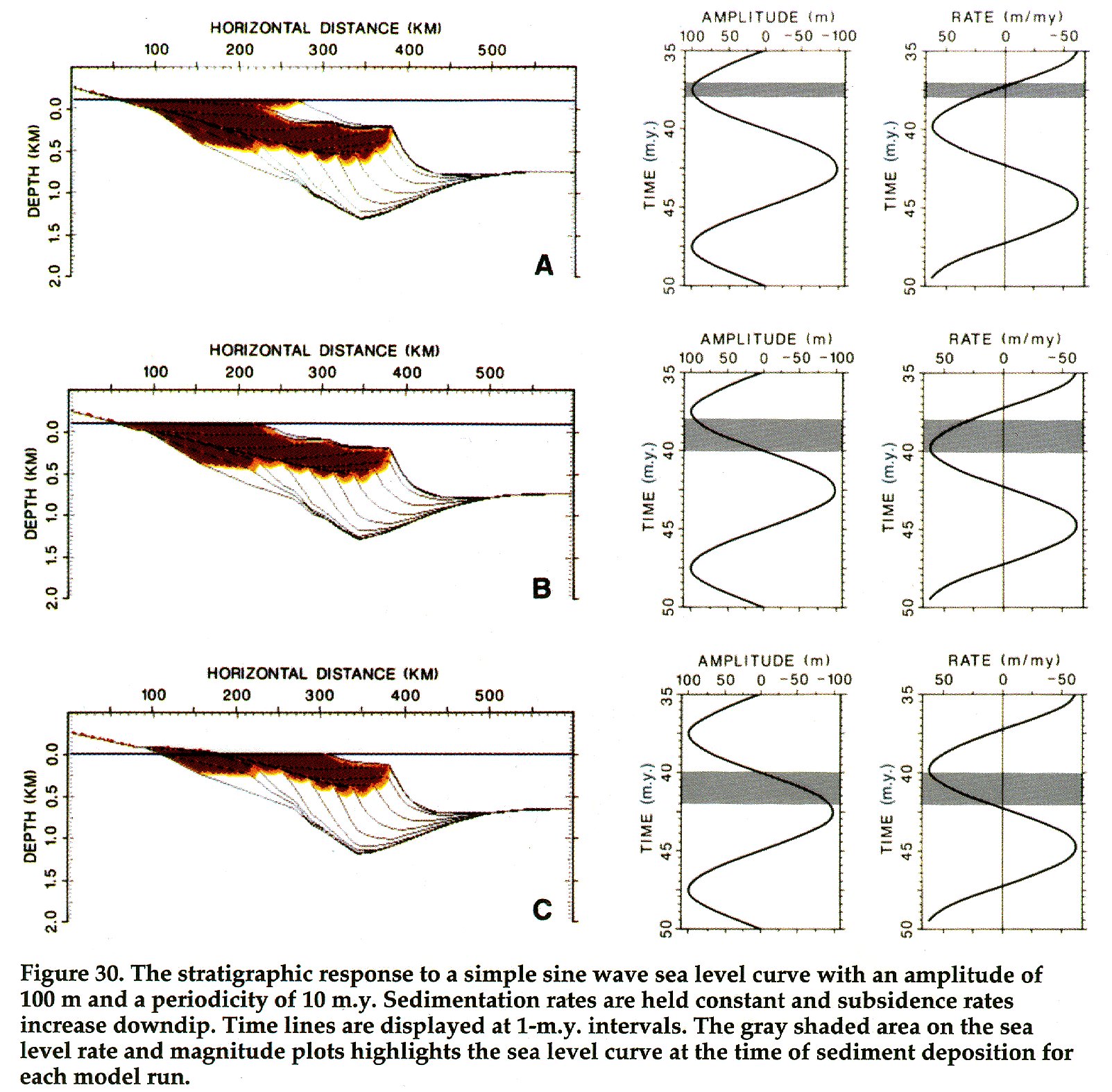
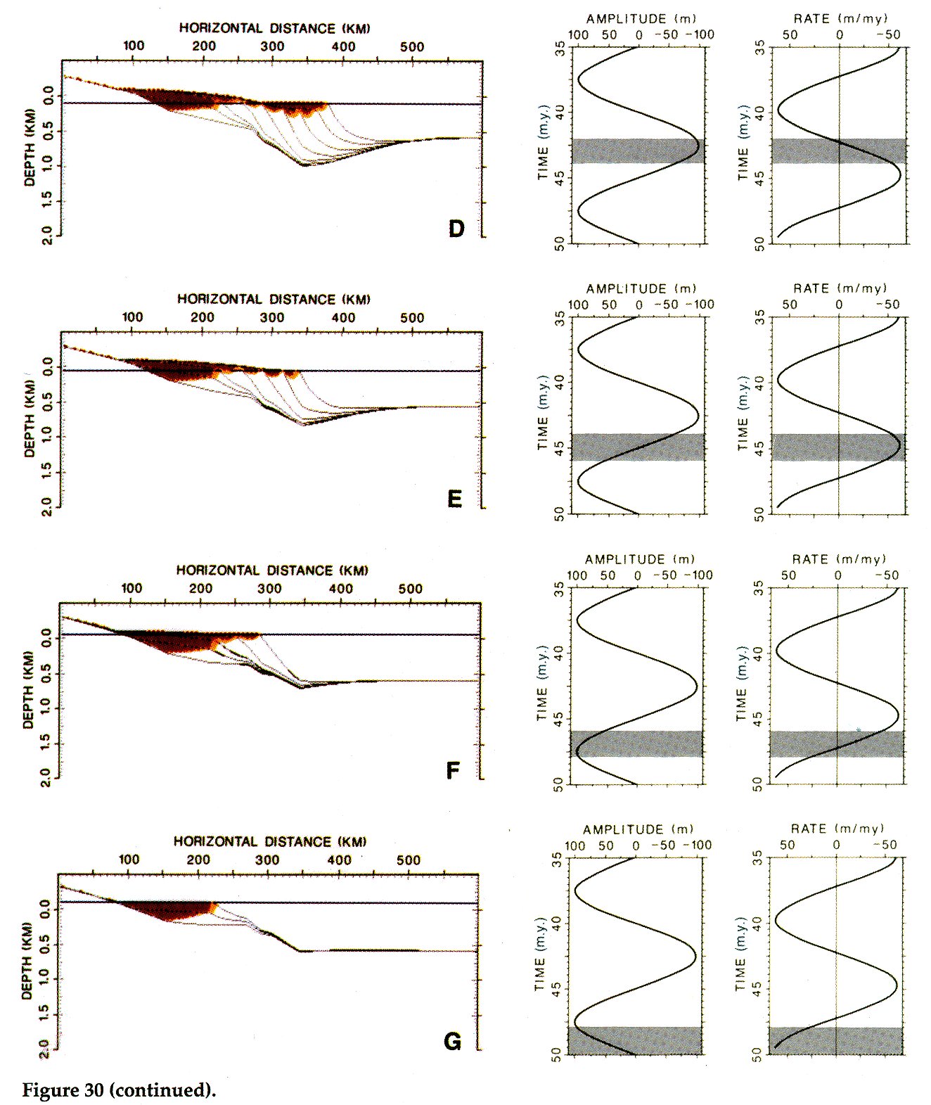
The stratigraphic response to a simple sine wave sea level curve with sedimentation rates held constant and subsidence rates increasing downdip is depicted in Figure 30 (case 17). This model is intended to demonstrate systems tract concepts. The actual stratigraphic response will vary from this ideal model as subsidence, sea level, and sediment input vary. The model shown assumes that all slopes are stable, and thus there is no bypass of sediment by slope failure. In Figure 30a, sea level is approaching a eustatic maximum, but the rate of sea level rise is beginning to slow down. A sigmoid progradational geometry is produced. Note that the shoreline is prograding seaward even while sea level is rising. Maximum transgressions do not correspond with maximum sea level rise unless a basin is sediment starved and subsidence rates are minimal. As sea level reaches its maximum level and starts to fall (Figure 30b), topsets thin, onlap is below the limit of seismic resolution, and the shoreline progrades rapidly seaward. The sequence boundary (Figure 30c) forms during the maximum rate of fall. Erosion at this point may remove some of the thin topsets deposited earlier. At the eustatic lowstand (Figure 30d), the rate of fall has slowed. When coupled with subsidence, this produces initial

Table 4. Subsidence rate data for cases 9 and 10.

End_Page 355------------------------

Click to view image in JPEG format. Fig. 22. [Color] Model stratigraphic evolution of a basin with constant sediment input and sea level, and variable subsidence rates with time and basin position (case 9). See Table 4 for subsidence input parameters. Basin is shown at 1-m.y. time intervals.

End_Page 356------------------------

aggradation of sediments and onlap at the shelf margin. As sea level begins to rise (Figure 30e), the shoreline initially continues to prograde, but then retreats rapidly landward as the rate of rise increases. Note that the maximum regression does not correspond to the eustatic sea level lowstand in a basin with abundant sediment supply. At the maximum rate of sea level rise (Figure 30f), the shelf is sediment starved and clastic sediments are trapped updip. Finally, as the eustatic maximum is approached, the rate of rise slows down and the system progrades seaward once again.

Figure 31 shows the stratigraphic response to four cycles of sea level change within a thermally subsiding basin. In this model, lowstand systems tracts, transgressive systems tracts, and highstand systems tracts (Van Wagoner et al., 1987; Posamentier and Vail, 1988) are well reproduced. Sedimentation rates were held constant during the simulation. Note that in this basin, with abundant sediment supply and relatively slow rates of sea level rise, the transgressive systems tract is quite thick. The downlap surface forms in the middle of the shelfal portion of the depositional sequence. In basins with limited sediment supply and very low-relief coastal plains, small rises in sea level may flood vast areas, and the transgressive systems tract will be much thinner.

CONCLUSIONS

This chapter has presented an analysis of sediment input rate, sea level, and subsidence as fundamental controls on sequence geometries. Changes in paleobathymetry commonly are confused with changes in relative sea level. A simple model with eustatic sea level held constant illustrates coeval shallowing and deepening in a single basin. Coarsening-upward fringe and shoreface sequences should be interpreted

Click to view image in JPEG format. Fig. 23. [Color] Detailed lithostratigraphy (at 0 Ma) and time blocks (each 1-m.y. interval shaded) for basin in Figure 22.

End_Page 357------------------------

Click to view image in JPEG format. Fig. 24. [Color] Modeled stratigraphic evolution of a basin with constant sediment input, variable subsidence rates with time and basin position (same as in Figure 22, case 9, Table 4), and a variable sea level history (see Figure 25).

End_Page 358------------------------

as shallowing upward, but should not necessarily be interpreted as evidence of relative sea level fall.

In the absence of any change in subsidence, sea level, or sedimentation rate, a clastic wedge prograding seaward on a passive margin will evolve from a sigmoid progradational to a sigmoid aggradational geometry. The farther the shoreline progrades, the more difficult it is for the shoreline to prograde.

An increase in the available volume of sediment produces progradation and simple updip thinning of sediments in a subsiding basin in the absence of any eustatic sea level change. Falling relative sea level is required to produce erosional toplap and downward shifts in coastal onlap. The maximum point of load-induced subsidence is transferred downdip as the system progrades, whereas areas updip of the load experience lower subsidence rates or are even slightly uplifted. This effect may be pronounced on elastically weak crust or on systems prograding over a mobile substrate. Load-induced toplap may be differentiated from sea level-induced toplap by anomalously steep dip of topset sediments in the case of load-induced toplap.

Onlap may be produced in several ways. Over-steepened slopes may bypass sediment even during periods of constant eustatic sea level (see case 1) or rising sea level with very high sediment input rates. The bypassed sediment may be deposited on an older slump scar or previously unstable slope, producing apparent onlap. During sea level falls, minimal space is available for sediment deposition on the shelf and coast, and consequently more sediment bypasses the shelf (via canyons, gorges, and slumps) and onlaps the base of the slope. Coastal onlap is produced by a rise in relative sea level in a basin. Even with constant eustatic sea level, relative sea level will rise in a subsiding basin. Coastal onlap is not produced by transgressions caused by a reduction in sediment input alone.

Downlap, transgressions and regressions, and slope bypass are not by themselves diagnostic of sea level change. Changes in sediment supply relative to the rate of space creation in the basin may produce these features. Sequences with seaward migration (progradation) of the shoreline, coupled with aggradation of topsets, were deposited during periods of rising relative sea level. In a subsiding basin, seaward migration of the shoreline with no preserved topsets indicates falling eustatic sea level.

Load-induced subsidence on relatively weak crust may produce stratal geometries that are easily misinterpreted. Topsets may be oversteepened by downdip load. Lateral variation in sediment load is expected to produce local variations in the amount of onlap, which will complicate estimates of the magnitude of sea level change.

Ambiguities in interpreting relative sea level from two-dimensional lines may be reduced in many cases by incorporating three-dimensional data. For example, in three dimensions, erosion and marked downcutting in the nonmarine section may indicate lowering of relative sea level. Large changes in sediment thickness along strike will point toward shifting depocenters.

For subsiding basins with moderate to high sediment supply, maximum transgression typically will take place prior to a eustatic sea level highstand, and maximum regression will take place after a sea level lowstand. Preservation of thick topset sequences implies rising relative sea level even during major regressions. Erosional sequence boundaries are most likely to form during the maximum rate of sea level fall.

The age of sequence boundaries will be synchronous (within the limits of biostratigraphic resolution) only if rates of sea level fall are much greater than rates of subsidence in all basins being correlated. The geographic and temporal extent of unconformities is much greater in slowly subsiding basins than in rapidly subsiding basins. The slower the rate of sea level fall, the greater the disparity in the age of unconformities between two basins with different subsidence histories, even though the sea level signals are identical. As the rate of sea level fall declines, some unconformities will be absent in rapidly subsiding basins. The near synchroneity of many sequences implies rapid rates of fall. Basins with different rates of sediment supply but similar subsidence histories will ave nearly synchronous sequence boundaries if the sea level history is the same for the two basins.

Fig. 25. Sea level curve used to model basin in Figure 24.

End_Page 359------------------------

Click to view image in JPEG format. Fig. 26. [Color] Detailed lithostratigraphy (at 0 Ma) and time blocks (each 1-m.y. interval shaded) for the basin in Figure 24.

Click to view image in JPEG format. Fig. 27. [Color] (A) Modeled stratigraphy for basin with slow subsidence, moderate sedimentation rate, and the Haq et al. (1987) sea level curve; red letter "B" identifies bypass zones on final time step bathymetry; red letter "S" identifies stable slopes; (B) modeled stratigraphy for a basin with the same input parameters as in (A), but with a much more rapid subsidence rate; (C) modeled stratigraphy with the same subsidence rate as the basin in (B), but with double the sedimentation rate.

Fig. 28. Chronostratigraphic plot of unconformities for the basins in Figures 27A (solid gray) and B (diagonal lines). Note that the regions of solid gray and diagonal lines represent unconformities and not sediment in the basin. Rates and magnitudes of sea level change used in the model are also presented.

Fig. 29. Chronostratigraphic plot of unconformities for the basins in Figures 27B (shaded regions) and C (diagonal lines). Note that the regions of solid gray and diagonal lines represent unconformities and not sediment in the basin. Rates and magnitudes of sea level change used in the model are also presented.

Click to view image in JPEG format. Fig. 30. [Color] The stratigraphic response to a simple sine wave sea level curve with an amplitude of 100 m and a periodicity of 10 m.y. Sedimentation rates are held constant and subsidence rates increase downdip. Time lines are displayed at 1-m.y. intervals. The gray shaded area on the sea level rate and magnitude plots highlights the sea level curve at the time of sediment deposition for each model run.

Click to view image in JPEG format. Fig. 30. [Color] Continued.

Click to view image in JPEG format. Fig. 31. [Color] Systems tract model illustrating the stratigraphic response to four cycles of sea level change within a thermally subsiding basin. Sediment volume is held constant in the model. Slope instability is included. Dotted lines represent sequence boundaries.

References:

Aigner, T., and H.E. Reineck, 1982, Proximality trends in modern storm sands from the Helgoland Bight (North Sea) and their implications for basin analysis: Senckenbergiana Maritima, v. 14, p. 183-215.
Aigner, T., M. Doyle, D. Lawrence, M. Epting, A. van Vliet, 1988, Quantitative modeling of carbonate platforms: some examples: SEPM Special Publication 44, p. 27-37.
Aigner, T., A. Brandenburg, A. van Vliet, M. Doyle, D. Lawrence, and J. Westrich, 1990, Stratigraphic modeling of epicontinental basins: two applications: Sedimentary Geology, v. 69, p. 167-190.
Allen, J., 1978, Studies in fluviatile sedimentation: an exploratory quantitative model for the architecture of avulsion-controlled alluvial suites: Sedimentary Geology, v. 21, p. 129-147.
Bates, C.C., 1953, Rational theory of delta formation: AAPG Bulletin, v. 37, p. 2119-2162.
Bonham-Carter, G., and A. Sutherland, 1967, Diffusion and settling of sediments at river mouths: a computer simulation model: Trans-actions Gulf Coast Association Geological Societies, v. 17, p. 326-338.
Brenchley, P J., 1985, Storm influenced sandstone beds: Modern Geology, v. 9, p. 369-396.
Bridge, J., and M., Leeder, 1979, A simulation model of alluvial stratigraphy: Sedimentology, v. 26, p. 617-644.
Bryant, W.R., P. Cernock, and J. Morelock, 1967, Shear strength and consolidation characteristics of marine sediments, in A.F. Richards, ed., Marine geotechnique: Urbana, Illinois, University of Illinois Press, p. 41-62.
Burton, R., C.G.St.C. Kendall, and I. Lerche, 1987, Out of our depth: on the impossibility of fathoming eustasy from the stratigraphic record: Earth-Science Reviews, v. 24, p. 237-277.
Butcher, S.W., 1990, The nickpoint concept and its
End_Page 360------------------------
Fig. 27. See caption on page 360.
End_Page 361------------------------
implications regarding onlap to the stratigraphic record, in T.A. Cross, ed., Quantitative dynamic stratigraphy: Englewood Cliffs, New Jersey, Prentice-Hall, p. 375-387.
Christie-Blick, N., 1991, Onlap, offlap and the origin of unconformity-bounded depositional sequences: Marine Geology, v. 97, p. 35-56.
Cochran, J., 1980, Some remarks on isostasy and the long-term behaviour of the continental lithosphere: Earth and Planetary Science Letters, v. 46, p. 266-274.
Coleman, J.M., 1981, Deltas: processes of deposition and models for exploration (2d ed.): Minneapolis, Minnesota, Burgess, 124 p.
Coleman, J.M., D.B. Prior, and J.F. Lindsay, 1983, Deltaic influences on shelf edge instability processes: SEPM Special Publication 33, p. 121-137.
Curray, J.R., 1964, Transgressions and regressions, in R.L. Miller, ed., Papers in marine geology: New York, Macmillan, p. 175-203.
Dailly, G.C., 1975, Some remarks on regression and transgression in deltaic sediments, in C.J. Vorath, E.R. Parker, and D.J. Glass, eds., Canada's continental margins and offshore petroleum exploration:
Fig. 28. See caption on page 360.
Fig. 29. See caption on page 360.
End_Page 362------------------------
Canadian Petroleum Geologists Bulletin, v. 24, p. 92-116.
Davis, R.A., and R.L. Ethington, 1976, Beach and nearshore sedimentation: SEPM Special Publication 24, 187 p.
Dutta, N.C., 1987, Fluid flow in low permeable porous media, in B. Doligez, ed., Migration of hydrocarbons in sedimentary basins: Paris, Editions Technip., p. 567-595.
Elliot, T., 1978, Deltas (Chapter 6) and Clastic Shorelines (Chapter 7), in H. G. Reading, ed., Sedimentary environments and facies: New York, Elsevier, p. 97-177.
Featherstone, B., T. Aigner, L. Brown, M. King, and W. Leu, 1991, Stratigraphic modeling of the Gippsland basin: APEA Journal, p. 105-114.
Flemings, P., and T. Jordan, 1989, A synthetic stratigraphic model of foreland basin development: Journal of Geophysical Research, v. 94, p. 3851-3866.
Frohlich, C., and R.K. Matthews, 1991, strata-various: a flexible Fortran program for dynamic forward modeling of stratigraphy, in E.K. Franseen, W.L. Watney, C.G.St.C. Kendall, and W.C. Ross, eds., Sedimentary modeling: computer simulations and methods for improved parameter definition: Kansas Geological Survey Bulletin 233, p. 449-463.
Galloway, W.E., 1989, Genetic stratigraphic sequences in basin analysis, architecture and genesis of flooding surface bounded depositional units: AAPG Bulletin, v. 73, p. 125-142.
Goodwin, P W., and E.J. Anderson, 1985, Punctuated aggradational cycles: a general hypothesis of episodic stratigraphic accumulation: Journal of Geology, v. 93, p. 515-533.
Grabau, A.W., 1913, Principles of stratigraphy: New York, A. G. Seiler, 1185 p.
Haq, B., J. Hardenbol, and P. Vail, 1987, Chronology of fluctuating sea levels since the Triassic: Science, v. 235, p. 1156-1166.
Harms, J.C., J.B. Southard, and R.G. Walker, 1982, Structures and sequences in clastic rocks: SEPM Short Course Notes No. 9, p. 1:1-8:51.
Heward, A., 1981, A review of wave-dominated clastic shoreline deposits: Earth-Science Review, v. 17, p. 233-276.
Hubbard, R.J., 1988, Age and significance of sequence boundaries on Jurassic and Early Cretaceous rifted margins: AAPG Bulletin, v. 72, p. 49-72.
Jervey, M.T., 1988, Quantitative geological modeling of siliciclastic rock sequences and their seismic expression, in C. Wilgus, ed., Sea level changes-an integrated approach: SEPM Special Publication 42, p. 47-69.
Karner, G., M. Steckler, and J. Thorne, 1983, Long-term thermo-mechanical properties of the continental lithosphere: Nature, v. 304, p. 250-253.
Keller, G. H., and D.N. Lambert, 1979, Geotechnical properties of continental slope deposits--Cape Hatteras to Hydrographer Canyon, in L.J. Doyle and O.H. Pilke, eds., Geology of continental slopes: SEPM Special Publication 27, p. 131-151.
Kendall, C.G.St. C., P. Moore, J. Strobel, R. Cannon, M. Perlmutter, J. Bezsdek, and G. Biswas, 1991, Simulation of the sedimentary fill of basins, in E.K. Franseen, W.L. Watney, C.G.St.C. Kendall, and W.C. Ross, eds., Sedimentary modeling: computer simulations and methods for improved parameter definition: Kansas Geological Survey Bulletin 233, p. 9-33.
Kenyon, P.M., and D.L. Turcotte, 1985, Morphology of a delta prograding by bulk sediment transport: GSA Bulletin, v. 96, p. 1457-1465.
Komar, P.D., 1976, Beach processes and sedimentation: Englewood Cliffs, New Jersey, Prentice-Hall, 429 p.
Kuznir, N., and G. Karner, 1985, Dependence of the flexural rigidity of the continental lithosphere on rheology and temperature: Nature, v. 316, p. 138-142.
Lawrence, D.T., M. Doyle, S. Snelson, and W.T. Horsfield, 1987, Stratigraphic modeling of sedimentary basins (expanded abstract): SEG 57th Annual International Meeting Expanded Abstracts Volume, p. 407-408.
Lawrence, D.T., M. Doyle, and T. Aigner, 1990, Stratigraphic simulation of sedimentary basins: concepts and calibration: AAPG Bulletin, v. 74, p. 273-295.
Leopold, L.B., and Maddock, T., 1953, Hydraulic geometry of stream channels and some physiographic implications: U.S. Geological Survey Professional Paper 252, 57 p.
Leopold, I.B., M.G. Wolman, and J.P. Miller, 1964, Fluvial processes in geomorphology: San Francisco, W. H. Freeman, 522 p.
McCubbin, D.G., 1982, Barrier island and strand plain facies, in P.A. Scholle and D. Spearing, eds., Sandstone depositional environments: AAPG Memoir 31, p. 247-280.
Muller, G., 1966, The new Rhine Delta in Lake Constance, in M.L. Shirley and J.E. Ragsdale, eds., Deltas in their geologic framework: Houston, Houston Geological Society, p. 107-124.
Pitman, W.C., 1978, Relationship between eustasy and stratigraphic sequences at passive margins: Geological Society of America Bulletin, v. 80, p. 1389-1403.
Pitman, W., and X. Golovchenko, 1983, The effect of sea level change on the shelf-edge and slope of passive margins: SEPM Special Publication 33, p. 41-58.
Posamentier, H., and P.R. Vail, 1988, Eustatic control on clastic deposition II--sequence and systems tract models, in C. Wilgus, ed., Sea level changes--an integrated approach: SEPM Special Publication 42, p. 125-154.
Posamentier, H., M.T. Jervey, and P.R. Vail, 1988, Eustatic controls on clastic deposition I--conceptual framework, in C. Wilgus, ed., Sea level changes--an integrated approach: SEPM Special Publication 42, p. 109-124.
Reineck, H.E., and I.B. Singh, 1980, Depositional sedimentary environments (2d ed.): New York, Springer-Verlag, 549 p.
Roberts, H.H., J.N. Suhayda, and J. M. Coleman, 1980, Sediment deformation and transport on low-angle
End_Page 363------------------------
slopes: Mississippi Delta, in D.R. Coates and J.D. Vitek, eds., Thresholds in geomorphology: London, Allen and Unwin, p. 131-167.
Ross, W.C., 1990, Modeling base-level dynamics as a control on basin-fill geometries and facies distribution--a conceptual framework, in T.A. Cross, ed., Quantitative dynamic stratigraphy: Englewood Cliffs, New Jersey, Prentice-Hall, p. 387-399.
Ross, W.C., 1991, Cyclic stratigraphy, sequence stratigraphy and stratigraphic modeling from 1964 to 1989: 25 years of progress? in E.K. Franseen, W.L. Watney, C.G.St.C. Kendall, and W.C. Ross, eds., Sedimentary modeling: computer simulations and methods for improved parameter definition: Kansas Geological Survey Bulletin 233, p. 3-8.
Scruton, P.G., 1960, Delta building and the delta sequence, in F.P. Shepard, F.B. Phleger, and T.J.H. Van Andel, eds., Recent sediments, northwest Gulf of Mexico: AAPG Bulletin, v. 44, p. 82-102.
Shuster, M.W., and D.W. Childers, 1992, High-resolution stratigraphy forward modeling: a case study of the Lower-Middle San Andres sequence, Permian Basin: AAPG Annual Convention Program and Abstracts, June 21-24, Calgary, p. 119.
Shuster, M.W., and D.T. Lawrence, 1991, Controls on passive margin stratigraphy: seismostratigraphic and basin modeling evaluation of Georges Bank Basin: AAPG Bulletin, v. 75, p. 671-672.
Summerhayes, C.P., 1986, Sea level curves based on seismic stratigraphy: their chronostratigraphic significance: Paleogeography, Paleoclimatology, Paleoecology, v. 57, p. 27-42.
Terzaghi, K., 1956, Varieties of submarine slope failures: Harvard Soil Mechanics Series, No. 52,
Fig. 30. See caption on page 360.
End_Page 364------------------------
reprinted from Publication 52, Norwegian Geotech. Inst., p. 1-16.
Thorne, J.A., 1985, Studies in stratology: the physics of stratigraphy: Ph.D. thesis, New York, Columbia University, 523 p.
Vail, P.R., 1987, Seismic stratigraphy interpretation procedure, in A.W. Bally, ed., Atlas of seismic stratigraphy: AAPG Studies in Geology 27, p. 1-10.
Vail, P.R., R.M. Mitchum, R.G. Todd, J.M. Widmier, S. Thompson III, J.B. Sangree, J.N. Bibb, and W.G. Hatelid, 1977, Seismic stratigraphy and global changes in sea level, in C.E. Payton, ed., Seismic stratigraphy--applications to hydrocarbon exploration: AAPG Memoir 26, p. 49-212.
Van Hinte, J.E., 1978, Geohistory analysis--application of micropaleontology in exploration geology: AAPG Bulletin, v. 62, p. 201-222.
Van Wagoner, J.C., R.M. Mitchum, Jr., H.W.
End_Page 365------------------------
Fig. 31. See caption on page 360.
End_Page 366------------------------
Posamentier, and P.R. Vail, 1987, Key definitions of sequence stratigraphy, in A.W. Bally, ed., Atlas of seismic stratigraphy: AAPG Studies in Geology 27, p. 11-14.
Watts, A., G. Karner, and M. Steckler, 1982, Lithospheric flexure and the evolution of sedimentary basins: Royal Society of London Philosophic Transactions, Series A, v. 305, p. 249-281.
Watts, A.B., and J.A. Thorne, 1984, Tectonics, global changes in sea level and their relationship to stratigraphic sequences at the U.S. Atlantic continental margin: Marine and Petroleum Geology, v. 1, p. 319-339.
Wright, L.D., and J.M. Coleman, 1972, River delta morphology: wave climate and the role of the subaqueous profile: Science, v. 176, p. 282-284.
Wright, L.D., and J.M. Coleman, 1974, Mississippi River mouth processes: effluent dynamics and morphological development: Journal of Geology, v. 82, p. 751-758.
End_of_Record - Last_Page 367-------
Acknowledgments:
This chapter was greatly improved by the constructive reviews of Bill Ross, Mark Shuster, Lyn Watney, Steve Tennant, Chuck Minero, and Dean Malouta. I thank Shell Oil Company for permission to publish this material.
Pay-Per-View Purchase Options
The article is available through a document delivery service. Explain these Purchase Options.