INTRODUCTION

Fault zones are generally recognized as being composed of a central fault core of varying thickness surrounded by a volume of deformed host rock or damage zone (Caine et al., 1996; Wibberley et al., 2008; Braathen et al., 2009). In rocks with porosities exceeding 10%–15%, damage zones are commonly characterized by deformation bands, which are millimeter- to centimeter-thick tabular zones derived from strain localization (Aydin, 1978; Wong et al., 1997; Fossen et al., 2007). In the present study, such damage zones, chiefly exhibiting deformation bands, are labeled “deformation band damage zones” to distinguish them from damage zones in lower-porosity rocks, which are dominated by fractures.

Cataclastic deformation bands are commonly associated with a reduction in porosity and permeability relative to their surrounding host rock (Antonellini and Aydin, 1994; Torabi et al., 2013). Deformation bands commonly display conjugate geometries in cross section, with one set being parallel to the main slip plane and the other dipping in the opposite direction (Shipton and Cowie, 2001, 2003; Berg and Skar, 2005; Fossen et al., 2007; Johansen and Fossen, 2008). Map views of outcrops show that deformation bands are not strictly parallel to one another but form reticular networks with lozenge-shaped bodies of host rock between deformation bands (Antonellini and Aydin, 1995; Shipton and Cowie, 2001; Awdal et al., 2014). Forming interconnected networks, deformation bands can induce order-of-magnitude effective permeability reductions and anisotropies (Antonellini and Aydin, 1994; Matthäi et al., 1998; Taylor and Pollard, 2000; Sternlof et al., 2004; Fossen and Bale, 2007; Rotevatn et al., 2009). Deformation band frequency varies throughout the damage zone, generally decreasing away from the fault core. The effect of deformation bands on reservoir fluid flow has been addressed by some previous studies using reservoir simulation tools (Rotevatn et al., 2009; Fachri et al., 2013a). Their results suggest that the presence of deformation bands with a permeability reduction of three orders of magnitude or more relative to the host rock increases flow tortuosity and enhances sweep efficiency, which in turn delays water breakthrough and increases oil recovery. In sum, heterogeneity and anisotropy introduced by deformation bands give rise to complex flow patterns, which influence reservoir behavior. Consequently, these features should be included in models employed for hydrocarbon production planning.

Fault damage zones are not routinely incorporated into industrial reservoir models. This is partly because of the existing modeling convention of representing faults as single planes rather than deformed rock volumes (Tveranger et al., 2004, 2005; Manzocchi et al., 2008, 2010), and also because of a lack of systematic, quantified descriptions of fault zones adapted for three-dimensional (3-D) modeling purposes (Braathen et al., 2009). A further obstacle is the difficulty of resolving and identifying fault zone details in seismic data. The practical consequence of this lack of direct observational evidence from the subsurface is that detailed fault zone models must be based on statistical data derived from outcrop studies. The commonly limited 3-D exposure of fault outcrops, however, dictates that data from multiple sites must be analyzed statistically to populate entire fault envelopes with properties. Furthermore, the modeled features need to be implemented at a suitable level of resolution, which, for larger models, precludes discrete rendering of individual features.

Compared with the more mature methods for characterization and modeling of sedimentary architectures and properties, the development of methods for characterizing and modeling structural heterogeneity is in its early stage. As a response to the need for more model-oriented methods for describing faults, Tveranger et al. (2005) proposed the concept of fault facies, which has subsequently been developed through several studies (Fredman et al., 2007, 2008; Cardozo et al., 2008; Braathen et al., 2009; Rotevatn et al., 2009; Fachri et al., 2011, 2013a, b; Schueller et al., 2013). Facies defined as “a body of rock with specific characteristics” (Middleton, 1978, p. 4) have traditionally been applied to descriptions of sedimentary rocks (Reading, 1986) and form the mainstay of 3-D geological modeling. The introduction of fault facies can be considered the natural extension of this concept into the realm of tectonized rock bodies. The utility of the facies approach lies in its flexibility for subdividing bodies of rock into distinct classes at any scale according to a specific set of properties or features: observed or interpreted (Braathen et al., 2009). As an example, deformation bands are the main structural component in damage zones in porous rocks, and deformation band density (number of deformation bands per meter) is a key property that can be quantified using scan lines from outcrops; thus, rocks in damage zones can be subdivided into classes according to deformation band density (Fachri et al., 2011, 2013a, b). Applying the fault facies concept, a database of quantified fault architecture parameters has been compiled, and some patterns regarding fault facies geometries, dimensions, and spatial distributions have been identified (Braathen et al., 2009; Schueller et al., 2013). Reservoir modeling methods that were originally developed for modeling sedimentary facies have been successfully employed for building fault facies models (e.g., Syversveen et al., 2006; Soleng et al., 2007; Fredman et al., 2008; Fachri et al., 2011, 2013a, b). Explicit modeling of small-scale heterogeneities of fault zones requires ultrahigh-resolution models. However, practical considerations regarding central processing unit cost favor the use of upscaled properties. Employing well-constrained fault facies for fault zone modeling may offer a flexible way of balancing current technical constraints and the need for including geological details.

Most previous models employing fault facies have been of limited size to allow the use of separate high-resolution fault zones. In these models, separate fault zone grids are generated from conventional reservoir models by extending 3-D grids around mapped fault planes. The procedure uses an algorithm implemented in the fault modeling software Havana. Fault zone grids are subsequently populated with properties using conventional reservoir modeling tools and merged back into the full reservoir model. At present this is not part of any standard workflow used by the petroleum industry but a prototype method developed for research purposes (e.g., Fredman et al., 2007, 2008; Soleng et al., 2007; Fachri et al., 2011; Qu et al., 2015).

The objective of this paper is to present a method for modeling permeability heterogeneity and anisotropy introduced by deformation bands in a reservoir-scale fault damage zone and a procedure for incorporating the fault damage zone in reservoir models. Our synthetic demonstration model includes the entire 3-D damage zone of a fault with maximum 100-m (328-ft) throw. Empirical data from extant studies are used to provide realistic constraints for the modeling process. Flow simulations are performed to investigate the resulting flow behavior and reservoir performance.

WORKFLOW OVERVIEW

The modeling workflow is summarized in Figure 1. It involves the following steps: (1) building the structural model, (2) generating a global grid and a fault zone grid and specifying extent of damage zone, (3) performing facies and petrophysical modeling on the global grid and fault zone grid separately, (4) merging the fault zone and global model, and (5) conducting flow simulation on the merged model. The present study focuses mainly on facies and petrophysical modeling performed on the fault zone model; the petrophysical properties of the surrounding global model were kept homogeneous and constant. Structural modeling, global grid generation, facies, and petrophysical modeling were performed in RMS (a reservoir modeling tool). Fault zone grid generation and merging of fault zone and global model were performed in Havana (fault modeling tool), and flow simulations were conducted using Eclipse (flow simulator).

Figure 1. Schematic workflow for the model building procedure. Shades indicate which software application was used in each step.

MODEL FRAMEWORK AND GRID

The structural model consists of a single, vertical fault aligned along the Y axis (Figure 2). The fault is initially defined as a conventional elliptic fault plane with a length of 1000 m (3280 ft) and a height of 500 m (1640 ft). Displacement ranges from 100 m (328 ft) at the center of the plane to 0 m at its edges. The top and bottom layers of the model are flat, outlining a model volume of 1000 × 1600 × 600 m (3280 × 5249 × 1968 ft) encasing the fault.

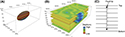Figure 2. Synthetic structural model employed in this study. The model measures 1000 × 1600 × 600 m (3280 × 5249 × 1968 ft). (A) The fault surface is 1000 m (3280 ft) long and extends 500 m (1640 ft) vertically. Displacement ranges from 100 m (328 ft) at the center of the plane to 0 m at its edges. (B) Layer model. The fault is completely encased by the top and bottom layers of the model, which are flat. Intervening layers are offset by the fault. (C) Illustration of an xz section from the middle of the model.

Using this structural framework, a conventional global grid with a resolution of 50 × 50 × 10 m (164 × 164 × 32.8 ft) was generated (Figure 3A). This global grid, including the fault plane, acts as input for generating the volumetric fault zone grid. The latter is to include the damage zone and comprises all cells adjacent to and up to a predefined distance away from the fault plane (Figure 3B). The generation of the fault zone grid is performed by an algorithm embedded in Havana, which allows the width and xyz resolution of the fault zone grid to be specified (Syversveen et al., 2006; Qu et al., 2015). In the present study, resolution of the fault zone grid is specified as 1 m (3.28 ft) in the fault-perpendicular (x) direction and 5 m (16.4 ft) in the fault-parallel (y) and the vertical (z) direction, yielding a total of 2.88 million cells.

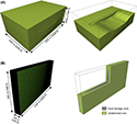Figure 3. Global grid and fault zone grid. (A) The global grid shown in different views. The dashed line indicates the area of the fault zone grid. (B) Fault zone grid generated from the global grid. Damage zone region is defined inside the fault zone grid.

The fault zone grid is intentionally made somewhat larger than the expected extent of the damage zone region to accommodate it. Thus, prior to performing property modeling, we need to specify which parts of the fault zone grid contain host rock and which belong to the damage zone. The extent of the latter is related to fault throw distribution. The damage zone width in the model is strongly dependent on which criteria are used for defining its outer boundary. Some workers employ a specified deformation band density to constrain the width of the damage zone (e.g., Berg and Skar, 2005; Schueller et al., 2013). According to Schueller et al. (2013), the damage zone width can be estimated from fault throw:

where W_1av is the average distance from the fault core to the farthest position at which the deformation band density is no lower than 1/m (/3.28 ft). T is the fault throw (available from the structural model). Equation 1 is employed here to define the extent of the damage zone region inside the fault zone grid, as illustrated in Figure 3B. The smooth, discus shape of the fault damage zone region results from the simplified assumption that the global model (i.e., stratigraphy) is homogeneous. In reality, the outline of the fault damage zone region is likely to be more irregular with damage zone width varying between stratigraphic units with different mechanical properties. However, our simplified model does serve to illustrate the expected trend where fault damage zone width conforms to fault throw distribution, i.e., decreasing from the center of the fault toward the fault tips. The maximum damage zone width in our model, corresponding to the maximum fault throw of 100 m (328 ft), is 71 m (232.9 ft). Property modeling inside the damage zone is outlined below. Cells outside the damage zone region (but inside the fault zone grid) are simply filled with host rock properties matching the global grid.

STOCHASTIC FAULT FACIES MODELING

Characterization

The characterization of fault facies employed here is based on data from Schueller et al. (2013). The data set consists of 106 outcrop scan lines from damage zones of extensional faults in porous sandstone and includes data from outcrop studies in Egypt, Utah, the United Kingdom, France, the Netherlands, and Svalbard. Scan line data record deformation band position and band density (i.e., number of deformation bands crossed per 1 m [3.28 ft]) along selected transects. The analysis of the data set carried out by Schueller et al. (2013) revealed a logarithmic decrease in deformation band density away from the fault core and a nonlinear relationship between damage zone width and fault throw (equation 1), which is adopted by us for defining damage zone width.

Here we approach the same data set from a different angle, aiming to implement the information into a sizable reservoir model with a limited resolution. To avoid explicit modeling of individual bands and enable the use of stochastic facies modeling extant in commercial reservoir modeling software, we define a discrete set of fault facies based on deformation band density. A similar approach has previously been employed by Fachri et al. (2013a, b).

The discretization of deformation band densities facilitates easy analysis of facies proportions, spatial relationship between facies, and facies continuity in the fault-perpendicular direction, which in turn can be used to set up a fault facies model.

Facies Classification and Their Proportion Trends

Six fault facies based on deformation band densities were initially defined: >20/m (/3.28 ft), 16–20/m (/3.28 ft), 11–15/m (/3.28 ft), 6–10/m (/3.28 ft), 1–5/m (/3.28 ft), and 0/m (/3.28 ft). The proportional spatial distribution of the different facies and their distance from the fault core were analyzed. Throw of the faults related to the data set by Schueller et al. (2013) mainly ranges between 0 and 300 m (0 and 984 ft). Damage zones related to larger fault throw are generally wider than those related to smaller faults. Thus, at the same distance from the fault core, facies proportions may differ. The data were therefore subdivided into three categories according to fault throw (<50 m [164 ft], 50–100 m [164–328 ft], and 100–300 m [328–984 ft]), and analysis of the relationship between facies proportions and distance from the fault core was carried out separately for each category. Results and functions used to calculate facies proportions are shown in Figure 4. The proportion of facies with deformation band density >20/m (/3.28 ft) ranges between 0.6 and 0.8 within 1-m (3.28-ft) distance from the fault core and decreases abruptly away from it. The proportions of facies with low deformation band density of 1–5/m (/3.28 ft) and 0/m (/3.28 ft) are very low close to the fault core and increase away from it. The proportions of the other facies do not exhibit any obvious trends and therefore remain relatively constant throughout the damage zone. Facies proportions are only marginally affected by fault throw at similar distances from the fault core. As shown in Figure 4, at the same distance from the fault core, the proportion of facies with deformation band density higher than 20/m (/3.28 ft) in the damage zones corresponding to fault throw category of <50 m (164 ft) is only slightly lower than that in the damage zones corresponding to larger fault throw.

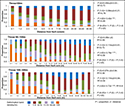Figure 4. Relationship between facies proportions and distance from the fault core related to three fault throw categories. The functions are listed on the right. P (>20), i.e., the proportion of facies with deformation band density >20/m (orange bar), decreases away from the fault core and shows a power law relationship with the distance to the fault core (d). P (1–5) and P (0), i.e., the proportions of facies with deformation band density 1–5/m (red bar) and 0/m (blue bar), are increasing away from the fault core and show logarithmic relationships with the distance to the fault core (d). The proportion of facies with deformation band density 6–20/m is more or less constant throughout the damage zone.

The proportion trends for facies with deformation band density >20/m (/3.28 ft), 1–5/m (/3.28 ft), and 0/m (/3.28 ft) were well defined by power law and logarithmic functions with high coefficients (Figure 4). To simplify modeling, facies with deformation band density of 6–10/m (/3.28 ft), 11–15/m (/3.28 ft), and 16–20/m (/3.28 ft) that did not show obvious proportion trend were merged into one facies with deformation band density of 6–20/m (/3.28 ft), and its relative proportion was described by the difference between 1 and the proportion of other facies. Thus, only four fault facies were ultimately used in the following modeling. These are labeled H (high deformation band density, >20/m [/3.28 ft]), M (medium deformation band density, 6–20/m [/3.28 ft]), L (low deformation band density, 1–5/m [/3.28 ft]), and U (undeformed, deformation band density of 0/m [/3.28 ft]).

Figure 5 shows the frequency distribution of deformation band density of facies H, facies M, and facies L. Facies H is composed of rock bodies with deformation band density higher than 20/m (/3.28 ft), and the deformation band density displays a power law distribution. The highest deformation band density of facies H observed in the data set is 160/m (/3.28 ft), whereas 90% of the data lie within the range of 20–70/m (/3.28 ft). The average deformation band density of this facies is 40/m (/3.28 ft). Deformation band density in facies M and facies L is evenly distributed, with average values of 11/m (/3.28 ft) and 3/m (/3.28 ft), respectively.

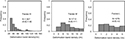Figure 5. Frequency distribution of deformation band density in different facies. AVE &equals; average; N &equals; number of observations.

Spatial Relationships between Facies

Spatial relationships between facies H, M, L, and U were analyzed as shown in Figure 6. Of 1241 facies contacts, 85% show a transition to neighboring facies classes (e.g., H/M, M/L, and L/U); facies H only rarely occurs adjacent to facies U. This observation is in accordance with Fachri et al. (2013b). The observed pattern suggests a laterally ordered spatial relationship between facies H, M, L, and U, which needs to be considered when populating the fault zone model with fault facies.

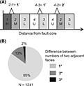Figure 6. Ordering of facies occurrence. (A) Illustration of facies distribution in a scan line measured from outcrops. Numbers 1, 2, 3, and 4 are assigned to facies H, M, L, and U, respectively. If two facies with successive numbers (e.g., H and M, M and L, and L and U) occur adjacent to each other, the difference between their assigned numbers is 1. (B) Frequency distribution of the difference between the numbers of two adjacent facies. N &equals; number of observations.

Continuity of Fault Facies

Analysis of the continuity of fault facies in a fault-perpendicular direction shows that 90% of individual facies bodies only extend for a distance of 1–5 m (3.3–16.4 ft) (Figure 7). Note that the statistical validity of this result is constrained by the input data of this study (i.e., faults with throw <300 m [984 ft]). Scatterplots of facies width versus fault throw show no close relationship between these two parameters, but a weak trend can be observed when employing a logarithmic scale (Figure 8).

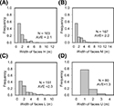Figure 7. Frequency distribution of the width of individual fault facies in a fault-perpendicular direction. (A) Facies H. (B) Facies M. (C) Facies L. (D) Facies U. AVE &equals; average; N &equals; number of observations.

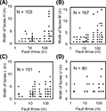Figure 8. Scatterplot of fault throw versus facies width in fault-perpendicular direction. (A) Facies H. (B) Facies M. (C) Facies L. (D) Facies U. N &equals; number of observations.

The continuity of the fault facies in a fault-parallel direction is more difficult to quantify. Measurement of deformation band lengths from Jurassic sandstones in southeastern Utah shows that the length of isolated deformation bands spans more than three orders of magnitude, from below 1 m (3.28 ft) to 100 m (328 ft) (Fossen and Hesthammer, 1997; Fossen et al., 2007). Because it is common that deformation bands overlap and interlink (Aydin, 1978; Sternlof et al., 2004; Fossen et al., 2007), the facies composed of bands are supposed to extend further than individual bands; thus, the length of isolated bands only hints at the minimum length of our fault facies in a fault parallel direction. A study of deformation band density at different localities along the Bartlett fault segment of the Moab fault in Utah (Berg and Skar, 2005) shows that the inner zone, which is close to the fault core with high deformation band density, is absent at some localities. At one locality, high deformation band density (30–50/m [/3.28 ft]) was observed close to the fault core, whereas approximately 100 m (328 ft) away, deformation band density close to the fault core is below 20/m (/3.28 ft). The estimated normal throw at the studies localities is between 170 and 300 m (558 and 984 ft) (Foxford et al., 1996; Berg and Skar, 2005). The distance between these two localities may provide a rough estimate of the maximum length of the fault parallel extent of the individual fault facies employed in our study. Based on the analysis above, the fault facies as defined in this paper are considered to extend from a couple a meters up to 100 m (328 ft) along the fault.

Modeling

The results from the analysis described above were used as input to populate the fault damage zone region with fault facies. Sequential indicator simulation (SIS) and truncated Gaussian simulation (TGS) have been used by other scientists for this purpose (Fachri et al., 2011, 2013a, b). When employing SIS, facies are modeled separately and independently, and possible constraints to their relative position are not considered (Journel and Alabert, 1990). It is applicable to cases with no interrelations between individual facies. The TGS can honor prior facies proportions and specific ordered transitions between facies. Facies are generated by truncating a simulated Gaussian field, as illustrated in Figure 9. The facies generated are in fixed sequence: facies k is (almost) never contiguous to facies k′ with k′ > k + 1 or k′ < k − 1. Prior information about the probability of facies k occurring at location u can be translated into a local threshold value t_k(u) (Xu, 1995). Application of this method for fault facies modeling was studied by Fachri et al. (2013a, b). In the present paper, TGS is employed for fault facies modeling. The main input in this step includes a 3-D fault zone grid, 3-D fault facies proportion trends, a variogram model of the Gaussian field, and a specification of the spatial order in which the facies occur.

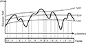Figure 9. Illustration of the generation of facies by truncating a simulated Gaussian field (the thick wavy curve) with some threshold curves t_k(u). u is location (modified from Xu, 1995).

The fault zone grid used to perform the fault facies modeling is generated from the global grid and includes the cells surrounding the fault plane. The choice of cell dimensions in the fault zone grid was made by considering the dimensions of the fault facies chosen for the modeling. In the fault-perpendicular direction, more than 90% of the fault facies extend within the range of 1 to 5 m (3.28 to 16.4 ft). Accordingly, the fault zone grid was constructed with cell dimension 1 m (3.28 ft) in the fault-perpendicular direction. The facies are elongated along the fault and are considered to extend a couple of meters to 100 m (328 ft). This gives more flexibility with respect to defining cell dimension in the fault-parallel direction. To keep a reasonably high resolution, fault-parallel (along y and z axes) cell dimensions were both set to 5 m (16.4 ft).

Variograms describe geometry and continuity of a variable (Gringarten and Deutsch, 2001). Figure 9 shows that the extents of the generated facies are controlled by both the threshold/proportion curves and the Gaussian field. The spatial statistics of the fault facies are complex functions of the input threshold curves t_k(u) and the variogram of the Gaussian field (Xu, 1995). A heuristic process can be implemented to obtain the set of input parameters (variogram model of the Gaussian field) that would yield a correct image of the facies spatial distribution (Xu, 1995). A spherical variogram model with range of 2 m (6.56 ft) in the x direction and 50 m (164 ft) in the y and z directions was used as a first approximation. Facies ordering from H to M, L, and U was specified.

The 3-D facies proportion trend parameters were generated using the proportion functions relating facies proportions to distance from the fault core and fault throw (Figure 10). The proportion of facies U was set to 1 outside the damage zone. At a particular location in the damage zone, these parameters control which fault facies are most likely to occur and in which directions the occurrence of a given fault facies increases or decreases (Fachri et al., 2013b).

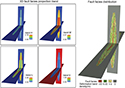Figure 10. Three-dimensional (3-D) facies proportion trend and an example of the resulting facies distribution after running the model. Facies H &equals; deformation band density >20/m (/3.28 ft); facies M &equals; deformation band density 6–20/m (/3.28 ft); facies L &equals; deformation band density 1–5/m (/3.28 ft); facies U &equals; undeformed rock.

Running the stochastic model produces a series of equiprobable 3-D fault facies distributions honoring the constraints defined by the model input (Figure 10). Facies H (in red) is mainly distributed in places close to the fault plane, surrounded by facies M (in green), which is occurring all over the damage zone. Facies U is mostly distributed outside the damage zone, with occasional presence within the damage zone adjacent to facies L or facies M. The continuity of individual facies in fault-perpendicular direction within the damage zone in the model is consistent with our outcrop data, with facies H and facies M extending within the range of 1–5 m (3.28–16.4 ft) and facies L and facies U mainly extending 1–3 m (3.28–9.84 ft). In a fault-parallel direction, facies extend from 5 m (16.4 ft) up to 100 m (328 ft), and facies H is more continuous close to the fault plane. These features are consistent with the outcrop observations; thus, the fault facies model generated with the current input setting is accepted.

Deformation band density models can then be produced based on the facies model, either by assigning a constant average deformation band density value for each facies or by assigning different deformation band density distributions to various facies. Figure 11 shows the deformation band density model generated in both ways. In the following sections, the petrophysical properties and flow simulation are performed based on the deformation band density model produced using the former approach.

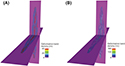Figure 11. Distribution of deformation band density in a fault damage zone generated by (A) assigning a constant average deformation band density value to each facies and (B) populating each facies with a range of values.

PETROPHYSICAL PROPERTIES

The petrophysical modeling centers on assigning permeability and porosity values to every cell in the fault damage zone model. The effective permeability of each cell is tied to the number of deformation bands in that cell. To calculate cell permeability in three directions (i.e., PermX, PermY, and PermZ), the number of deformation bands crossing imaginary scan lines in the x, y, and z directions in each cell is needed. This could not be extracted directly from the data set because most scan lines did not include detailed observation of deformation band orientation. The data set model provides deformation band density in fault-perpendicular (x) direction; however, deformation band density in fault-parallel (y) and vertical (z) direction are not available. Rotevatn et al. (2009) used the relationship between deformation band density in fault-parallel and fault-perpendicular direction to calculate the effective cell permeability in fault-parallel direction. For the purpose of the present study, the ratio between deformation band density in fault-parallel and fault-perpendicular direction and the ratio between deformation band density in vertical and fault-perpendicular direction in damage zones that associated to single normal faults were investigated using several published outcrop maps and sections (Table 1); deformation band orientations and dips were compiled, and the relationships between the ratios and the deformation band orientations and dips were analyzed.

The procedure used to analyze the number of deformation bands crossed per unit in different directions is illustrated in Figure 12. Square units with two sets of perpendicularly intersecting scan lines were placed on field maps and cross sections. The unit size is 0.5 × 0.5 m (1.64 × 1.64 ft) or 1 × 1 m (3.28 × 3.28 ft) and depends on the resolution of the map. Each set consists of five scan lines. One set of scan lines is perpendicular to the fault orientation, and the other set is parallel to the fault in the horizontal field map or vertical in the cross sections. In each square, the average number of deformation bands intersected by each set of scan lines was used to calculate the ratio of deformation band density in different directions. Also, the average intersection angle between deformation bands and fault orientation and the average dip angle of deformation bands in each square unit were recorded to analyze their relationship with the ratio of deformation band density in different directions.

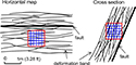Figure 12. Conceptual sketch showing the procedure used to analyze the number of deformation bands crossed per unit in different directions from horizontal maps and cross sections. Each square unit (shown in red) contains two sets of perpendicularly intersecting scan lines (blue lines). One set of scan lines is perpendicular to the fault orientation, and the other set is parallel to the fault in the horizontal map or vertical in the cross section. In each square unit, the number of deformation bands intersected along each set of scan lines was counted, and the ratio of deformation band density in different directions was calculated from the average number of deformation bands crossed along each set of scan lines. The average intersection angle between deformation bands and fault and the average deformation band dip angle in each square unit were recorded.

The ratio of deformation band density in fault-parallel and fault-perpendicular direction (parallel/perpendicular ratio for short) from 56 measurement units in horizontal field maps shows a narrow range between 0.07 and 0.25, with an average value of 0.15 (Figure 13A). The parallel/perpendicular ratio is positively correlated with the intersection angle (θ) between the deformation bands and the fault orientation (Figure 13B). The parallel/perpendicular ratio and the intersection angle (θ) display a relationship: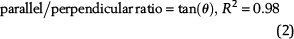

The ratio in our study is a bit lower compared with the ratio reported by Rotevatn et al. (2009) from a relay ramp structure in Utah, which is 0.2 in low deformation band density areas and 0.5 in high deformation band density areas. The difference may be caused by the fact that the relay ramp is formed by two interacting faults, which form a more complex network of crossover band sets across the relay ramp and therefore larger intersection angles than in the single fault damage zone modeled in this paper. The average parallel/perpendicular ratio in our study agrees well with a recent study of geometry of deformation band lozenges associated in extensional faults from Utah and Scotland by Awdal et al. (2014). Deformation band lozenges are rock volumes contained between deformation bands. They exhibit oblate-shaped geometry, with a long (x) axis parallel to the strike of deformation bands (length), an intermediate (y) axis parallel to the dip direction of the bands (height), and a short (z) axis normal to the strike of the deformation bands (thickness). The dimensions of these 3-D lozenges bounded by deformation bands reflect the deformation band spacing and deformation band density in different directions. Awdal et al. (2014) pointed out that the average ratio of length to the maximum thickness of a lozenge is 7.3, which implies that the average deformation band density in fault-parallel direction is 0.14 times the average deformation band density in the fault-perpendicular direction.

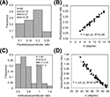Figure 13. The ratio of deformation band density in different directions and their relationships with deformation band orientations. (A) Frequency distribution of the ratio of deformation band density in fault-parallel direction to deformation band density in fault-perpendicular direction. (B) Scatterplot of the ratio of deformation band density in fault-parallel direction to deformation band density in fault-perpendicular direction versus the intersection angle (θ) between the deformation band orientation and fault orientation. (C) Frequency distribution of the ratio of deformation band density in vertical direction to deformation band density in fault-perpendicular direction. (D) Scatterplot of the ratio of deformation band density in vertical direction to deformation band density in fault-perpendicular direction versus the dip angle (α) of deformation bands. AVE &equals; average; MAX &equals; maximum; MIN &equals; minimum; N &equals; number of observations.

The ratio of deformation band density in vertical and fault-perpendicular direction (vertical/perpendicular ratio for short) from 46 measurement units in cross sections shows a wider range between 0.03–1.3, with an average value of 0.5. The vertical/perpendicular ratio displays a negative correlation with the dip angle (α) of deformation bands (Figure 13D), and these two variables show a relationship: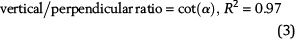

The parallel/perpendicular ratio range and the vertical/perpendicular ratio range were used to constrain the deformation band density in fault-parallel and vertical directions in our model. In our study, we consider an arrangement of nonvertical deformation bands with vertical/perpendicular ratio of 0.5 and parallel/perpendicular ratio of 0.15. Harmonic averaging method was used for calculating effective cell permeability in three directions, by assuming that deformation bands form continuous barriers to the imposed flow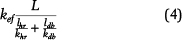



where k_ef is the effective permeability over the distance L, which is the cell length (1 m [3.28 ft] in the x direction); k_hr and k_db are the permeability of the host rock and deformation bands, respectively; l_hr and l_db are the accumulated thickness of the host rock and deformation bands over the distance L; and d is the thickness of an individual deformation band.

Constant deformation band density values were assigned to each facies. For deformation band density in fault-perpendicular direction, the median number of each facies was used: 40 db/m (/3.28 ft) for facies H, 11 db/m (/3.28 ft) for facies M, 3 db/m (/3.28 ft) for facies L, and 0 db/m (/3.28 ft) for facies U. Then the deformation band density in the fault-parallel direction was obtained by multiplying a parallel/perpendicular ratio of 0.15, and the deformation band density in the vertical direction was obtained by multiplying a vertical/perpendicular ratio of 0.5. The thickness of individual deformation bands was set to 2 mm (0.079 in.). Undeformed sandstone permeability was set to 1000 md horizontally, and 100 md vertically. Published studies state that permeability inside bands may be 0–6 orders of magnitude lower than the rock matrix (e.g., Antonellini and Aydin, 1994; Fisher and Knipe, 2001; Shipton et al., 2002; Torabi et al., 2013). We have selected values within this range and used band permeability of 10, 1, 0.1, and 0.01 md in our models. The calculated permeability values of each fault facies corresponding to different permeability scenarios are listed in Table 2. Permeability anisotropy is displayed because of the different number of deformation bands crossed in different directions. Under the scenarios defined in this paper, the permeability of fault facies containing deformation bands in the fault-parallel direction is shown to be 2–7 times higher than that in the fault-perpendicular direction.

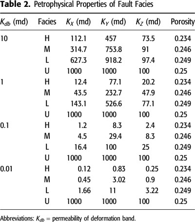
The arithmetic averaging method was used for calculating the effective porosity of each cell by setting the undeformed sandstone porosity to 0.25 and the deformation band porosity to 0.05. It shows that the low-porosity deformation bands did not cause significant reduction in the bulk porosity of fault facies (Table 2). This is because the volume fraction of deformation bands is small. For example, in fault facies with high deformation band density of 40/m (/3.28 ft), the volume fraction of deformation bands is just 8%.

FLOW SIMULATIONS

Flow simulations were performed on reservoir models containing damage zones. The aim was to address the following: (1) time needed to run simulations on a high-resolution fault zone model, (2) model response to introducing an explicit fault zone, and (3) possible errors caused by not including damage zone characterization in the models. In order to study the impact of including fault damage zones in the model, flow simulations employing different deformation band permeability settings (0.01, 0.1, 1, and 10 md) were carried out. A model without a damage zone (here termed “conventional model”) (Figure 14) served as a benchmark.

Figure 14. (A) Simulation model without damage zone. Fault is only represented as a two-dimensional surface. (B) Simulation model containing a volumetrically expressed fault damage zone, with internal permeability variations. The damage zone is merged with the global grid by replacing the cells enclosing the fault in the coarse global grid with a finer fault zone grid containing explicit properties.

Setup

In the global model, the top zone and the bottom zone were set to impermeable cap rock and floor rock seals, and the zones in between were defined as sandstone with horizontal permeability (x and y) of 1000 md, vertical permeability 100 md, and porosity 0.25. In the fault damage zone model, porosity and permeability values were assigned to each fault facies according to the calculated values listed in Table 2, and the rock volumes occupied by the cap and floor rocks were set to be impermeable by assuming they had deformed in a completely ductile manner. The fault damage zone model was then merged with the global model, replacing the part of the coarse global grid around the fault by a finer one with explicit fault damage zone properties (Figure 14).

Eclipse was used for water flooding simulation in an oil–water system. Initial oil saturation was set to 0.8 for the entire model. A vertical water injector was positioned in the hanging wall, and a vertical producer was placed in the footwall. All layers were perforated. Wells were controlled by predefined rate targets with pressure limits. All simulations were run until the water cut in the production well exceeded 90%. Details of rock, fluid, and production parameters are presented in Table 3. The relative permeability curve used for flow simulation is presented in Figure 15. The maximum time step was set to 10 days.

Figure 15. Relative permeability curve used for the flow simulations. K_r &equals; relative permeability; K_ro &equals; oil relative permeability; K_rw &equals; water relative permeability; S_w &equals; water saturation.

Fluid Flow Simulation Results

It took from 1 to 4 hr to complete the flow simulation using the reservoir models containing damage zones, as compared to 14 sec using the conventional model. No convergence problems were encountered.

Figures 16 and 17 show snapshots of the reservoir simulation in the conventional model and models including damage zones with different deformation band permeabilities. The model employing a deformation band permeability of 10 md shows similar flow behavior to the conventional model: the injected water crossed the fault and moves directly toward the producer without being deflected around the fault (Figure 16A, B). In the models with deformation band permeability of 1, 0.1, and 0.01 md, the cross-fault flow is baffled and redirected around the fault tips (Figure 16C–E). In the model employing a deformation band permeability of 0.01 md, the cross-fault flow was extremely inhibited, leaving undrained oil in the damage zone when the production well is abandoned (Figures 16E and 17E). This agrees with previous conclusions by Rotevatn et al. (2009), who concluded that the permeability contrast between matrix and deformation band permeability must exceed more than three orders of magnitude to significantly affect fluid flow.

Figure 16. Simulation results based on a single injector well–producer well pair. (A) Oil saturation after 1 yr and 2 yr of water injection and oil saturation at the end in a reservoir model without damage zone and reservoir models containing damage zones with deformation band permeability (K_db) of (B) 10 md, (C) 1 md, (D) 0.1 md, and (E) 0.01 md. Oil sat. &equals; oil saturation.

Figure 17. Cross-section view of (A) oil saturation after 2 yr of water injection and oil saturation at the end in a reservoir model without damage zone and reservoir models containing damage zones with deformation band permeability of (B) 10 md, (C) 1 md, (D) 0.1 md, and (E) 0.01 md. Injector is on the right side, and producer is on the left side. Oil sat. &equals; oil saturation.

Reservoir responses regarding time to water breakthrough, time to abandonment, and oil recovery were monitored for each simulation. Generally, the reservoir models containing damage zones showed different reservoir responses compared with the model without damage zone (Figure 18), e.g., later water breakthrough, earlier abandonment, and somewhat higher oil recovery. These differences become more pronounced as the permeability of deformation bands in the modeled damage zones decreases but reach a maximum when the permeability contrast between host rock and deformation band is four orders of magnitude. Similar findings are reported in Rotevatn et al. (2009). The time to water breakthrough is 140 days in the conventional model and 180, 300, 668, and 650 days in the reservoir models containing damage zones with deformation band permeability of 10, 1, 0.1, and 0.01 md, respectively (Figure 18A). This is because the low permeability of the deformation bands in the damage zones decreases the speed of the waterfront from the injection well and thereby delays the water breakthrough. The time to abandonment is 4383 days in the conventional model, compared with 4108, 3287, 2808, and 2788 days in the reservoir models containing damage zones with deformation band permeability of 10, 1, 0.1, and 0.01 md, respectively (Figure 18B). Differences in oil recovery factor are small: 0.62 for the conventional model compared with 0.64, 0.68, 0.7, and 0.7 in the models containing damage zones with deformation band permeability of 10, 1, 0.1, and 0.01md, respectively (Figure 18C).

Figure 18. Reservoir responses of models with and without damage zone. Models containing damage zones (indicated with the filled squares) apply deformation band permeabilities of 10, 1, 0.1, and 0.01 md. (A) Time to water breakthrough. (B) Time to abandonment. (C) Oil recovery at the end.

The snapshots of oil saturation at the end show that the remaining oil is distributed differently in these models (Figures 16 and 17). In the conventional model as well as in models with deformation band permeability higher than 0.01 md, the remaining oil is mainly distributed along the edges of the model. In contrast, in the reservoir model with deformation band permeability of 0.01 md, the damage zone exhibits remaining undrained oil volumes. A full study of the implications this may have for optimizing well positioning for production purposes is outside the scope of this paper, but initial testing suggests that horizontal wells positioned along the damage zone could enhance the recovery factor. Our study demonstrates that detailed representation of fault damage zone properties in reservoir models may both improve forecasting of reservoir behavior and aid production optimization.

DISCUSSION

Our model differs from previous fault facies studies (Syversveen et al., 2006; Fredman et al., 2007, 2008; Soleng et al., 2007; Fachri et al., 2011) in that we include a field-size full fault envelope with varying width in the reservoir model. This study uses a 3-D fault zone grid generation technique that allows property modeling on a discrete high-resolution fault zone grid separately from the global grid without refining the entire model. The input parameters for building the facies and petrophysical model of the damage zone are derived from statistical analysis of extensive outcrop data. This produces a more realistic model compared with previous models. The spatial distribution and extent of individual facies in fault-perpendicular direction is well constrained by an extensive data set. Some parameters have large uncertainties, e.g., the extent of fault facies in fault-parallel direction. The limited availability of 3-D outcrops constrains the quantification of fault facies extent in fault-parallel direction. It also highlights the necessity for targeted acquisition of specific outcrop data for improved modeling purposes. For parameters that have large uncertainties, additional sensitivity study will be performed to further unravel which parameters have significant influence on fluid flow and which parameters can be ignored.

The fault facies and deformation band density model provides a distribution of meter-scale heterogeneity introduced by the spatial variations of deformation band density within the fault damage zone. The millimeter- to centimeter-scale individual bands are not represented explicitly in our large-scale fault damage zone model because they are smaller than the grid resolution; thus, their orientation, thickness, and continuity cannot be captured directly. In the present paper, the effective cell permeability is calculated using harmonic averaging method considering an arrangement of deformation bands that completely transect the grid cell and form continuous barriers to the imposed flow. The orientation of bands is considered with the application of the ratio of deformation band density in different directions. The effective cell permeability calculated in this paper can be regarded as a minimum approximation. For more accurate approximation of effective permeability of cells holding discontinuous deformation bands, flow-based upscaling can be carried out on high-resolution minigrids with explicitly represented individual deformation bands (Sternlof et al., 2004). The upscaled permeability can be employed as input to fault facies or deformation band density model, which can be included in subsequent reservoir simulations. This is outside the scope of the present paper but part of an ongoing research effort.

CONCLUSIONS

We have generated a reservoir-scale 3-D model of a deformation band damage zone and presented a workflow for how to build it using standard industrial reservoir modeling tools. The model employs a generic geometry and properties derived from an extensive set of deformation band scan lines collected from extensional faults in sandstones. Property modeling of the damage zone was conducted using a standard two-step (facies + petrophysics) approach.

Four fault facies were defined by discretizing observed deformation band frequencies. Analysis of the discretized data revealed several features that were employed for conditioning spatial facies relationships in the model. The proportion of facies with high deformation band density decreases away from the fault core, and proportion of facies with low deformation band density increases away from the fault core. Facies with high deformation band densities nearly always occur adjacent to facies with medium deformation band density. Juxtaposition of facies with high deformation band density with facies with low deformation band density or undeformed rock is rare.

The fault facies patterns revealed when discretizing the scan line data are reproduced in the 3-D model using TGS. Deformation band densities in the x, y, and z directions were assigned to each facies considering band orientation. Petrophysical properties of each cell could then be calculated based on the deformation band density model.

Flow simulation of a selection of models shows that flow paths, sweep, and distribution of remaining oil can be substantially influenced by whether or not a damage zone is included in the model. Effect of the damage zone on flow patterns is closely linked to the permeability of the deformation bands in the damage zone. Lower permeability causes increased bypassing and trapping of oil in the damage zone. Reservoir models including damage zone properties exhibit different reservoir responses compared to models where the damage zone is not included. These contrasts become more pronounced as deformation band permeability decreases but reach a maximum when the permeability contrast between host rock and deformation band is four orders of magnitude.

REFERENCES CITED

Antonellini, M., and A. Aydin, 1994, Effect of faulting on fluid flow in porous sandstones: Petrophysical properties: AAPG Bulletin, v. 78, no. 3, p. 355–377.
Antonellini, M., and A. Aydin, 1995, Effect of faulting on fluid flow in porous sandstones: Geometry and spatial distribution: AAPG Bulletin, v. 79, no. 5, p. 642–670.
Awdal, A., D. Healy, and G. I. Alsop, 2014, Geometrical analysis of deformation band lozenges and their scaling relationships to fault lenses: Journal of Structural Geology, v. 66, 11–23, doi:10.1016/j.jsg.2014.05.006.
Aydin, A., 1978, Small faults formed as deformation bands in sandstone: Pure and Applied Geophysics, v. 116, p. 913–930, doi:10.1007/BF00876546.
Berg, S. S., and T. Skar, 2005, Controls on damage zone asymmetry of a normal fault zone: Outcrop analyses of a segment of the Moab fault, SE Utah: Journal of Structural Geology, v. 27, p. 1803–1822, doi:10.1016/j.jsg.2005.04.012.
Braathen, A., J. Tveranger, H. Fossen, T. Skar, N. Cardozo, S. Semshaug, E. Bastesen, and E. Sverdrup, 2009, Fault facies and its application to sandstone reservoirs: AAPG Bulletin, v. 93, no. 7, p. 891–917, doi:10.1306/03230908116.
Caine, J. S., J. P. Evans, and C. B. Forster, 1996, Fault zone architecture and permeability structure: Geology, v. 24, p. 1025–1028, doi:10.1130/0091-7613(1996)024<1025:FZAAPS>2.3.CO;2.
Cardozo, N., P. Røe, H. H. Soleng, N. Fredman, J. Tveranger, and S. Schueller, 2008, A methodology for efficiently populating faulted corner point grids with strain: Petroleum Geoscience, v. 14, p. 205–216, doi:10.1144/1354-079308-738.
Du Bernard, X., P. Labaume, C. Darcel, P. Davy, and O. Bour, 2002, Cataclastic slip band distribution in normal fault damage zones, Nubian sandstones, Suez rift: Journal of Geophysical Research, v. 107, p. 2156–2202.
Fachri, M., A. Rotevatn, and J. Tveranger, 2013a, Fluid flow in relay zones revisited: Towards an improved representation of small-scale structural heterogeneities in flow models: Marine and Petroleum Geology, v. 46, p. 144–164, doi:10.1016/j.marpetgeo.2013.05.016.
Fachri, M., J. Tveranger, A. Braathen, and S. Schueller, 2013b, Sensitivity of fluid flow to deformation-band damage zone heterogeneities: A study using fault facies and truncated Gaussian simulation: Journal of Structural Geology, v. 52, p. 60–79, doi:10.1016/j.jsg.2013.04.005.
Fachri, M., J. Tveranger, N. Cardozo, and O. Pettersen, 2011, The impact of fault envelope structure on fluid flow: A screening study using fault facies: AAPG Bulletin, v. 95, no. 4, p. 619–648, doi:10.1306/09131009132.
Fisher, Q., and R. Knipe, 2001, The permeability of faults within siliciclastic petroleum reservoirs of the North Sea and Norwegian Continental Shelf: Marine and Petroleum Geology, v. 18, p. 1063–1081, doi:10.1016/S0264-8172(01)00042-3.
Fossen, H., and A. Bale, 2007, Deformation bands and their influence on fluid flow: AAPG Bulletin, v. 91, no. 12, p. 1685–1700, doi:10.1306/07300706146.
Fossen, H., and J. Hesthammer, 1997, Geometric analysis and scaling relations of deformation bands in porous sandstone: Journal of Structural Geology, v. 19, p. 1479–1493, doi:10.1016/S0191-8141(97)00075-8.
Fossen, H., R. A. Schultz, Z. K. Shipton, and K. Mair, 2007, Deformation bands in sandstone: A review: Journal of the Geological Society, v. 164, p. 755–769, doi:10.1144/0016-76492006-036.
Foxford, K., I. Garden, S. Guscott, S. Burley, J. Lewis, J. Walsh, and J. Watterson, 1996, The field geology of the Moab Fault, in Huffman, A. C., Jr., W. R. Lund, and L. H. Godwin, eds., Geology and resources of the Paradox Basin: Salt Lake City, Utah, Utah Geological Association Guidebook 25, p. 265–283.
Fredman, N., J. Tveranger, N. Cardozo, A. Braathen, H. Soleng, P. Roe, A. Skorstad, and A. R. Syversveen, 2008, Fault facies modeling: Technique and approach for 3-D conditioning and modeling of faulted grids: AAPG Bulletin, v. 92, no. 11, p. 1457–1478, doi:10.1306/06090807073.
Fredman, N., J. Tveranger, S. Semshaug, A. Braathen, and E. Sverdrup, 2007, Sensitivity of fluid flow to fault core architecture and petrophysical properties of fault rocks in siliciclastic reservoirs: A synthetic fault model study: Petroleum Geoscience, v. 13, p. 305–320, doi:10.1144/1354-079306-721.
Gringarten, E., and C. V. Deutsch, 2001, Teacher’s aide variogram interpretation and modeling: Mathematical Geology, v. 33, p. 507–534, doi:10.1023/A:1011093014141.
Herrin, J. M., 2001, Characteristics of deformation bands in poorly lithified sands: Rio Grande rift, New Mexico, master’s thesis, New Mexico Institute of Mining and Technology, Socorro, New Mexico, 84 p.
Johansen, T. E. S., and H. Fossen, 2008, Internal geometry of fault damage zones in interbedded siliciclastic sediments: Geological Society, London, Special Publications 2008, v. 299, p. 35–56, doi:10.1144/SP299.3.
Journel, A. G., and F. G. Alabert, 1990, New method for reservoir mapping: Journal of Petroleum Technology, v. 42, p. 212–218, doi:10.2118/18324-PA.
Manzocchi, T., C. Childs, and J. Walsh, 2010, Faults and fault properties in hydrocarbon flow models: Geofluids, v. 10, p. 94–113.
Manzocchi, T., A. Heath, B. Palananthakumar, C. Childs, and J. Walsh, 2008, Faults in conventional flow simulation models: A consideration of representational assumptions and geological uncertainties: Petroleum Geoscience, v. 14, p. 91–110, doi:10.1144/1354-079306-775.
Matthäi, S., A. Aydin, D. Pollard, and S. Roberts, 1998, Numerical simulation of departures from radial drawdown in a faulted sandstone reservoir with joints and deformation bands: Geological Society, London, Special Publications 1998, v. 147, p. 157–191, doi:10.1144/GSL.SP.1998.147.01.11.
Middleton, G. V., 1978, Facies, in Fairbridge, R. W., and J. Bougeois, eds., Encyclopedia of sedimentology: Stroudsburg, Pennsylvania, Hutchinson & Ross, p. 323–325.
Qu, D., P. Røe, and J. Tveranger, 2015, A method for generating volumetric fault zone grids for pillar gridded reservoir models: Computers & Geosciences, v. 81, p. 28–37, doi:10.1016/j.cageo.2015.04.009.
Reading, H. G., 1986, Sedimentary environments and facies: Oxford, United Kingdom, Blackwell Scientific, 615 p.
Rotevatn, A., J. Tveranger, J. Howell, and H. Fossen, 2009, Dynamic investigation of the effect of a relay ramp on simulated fluid flow: Geocellular modeling of the Delicate Arch Ramp, Utah: Petroleum Geoscience, v. 15, p. 45–58, doi:10.1144/1354-079309-779.
Schueller, S., A. Braathen, H. Fossen, and J. Tveranger, 2013, Spatial distribution of deformation bands in damage zones of extensional faults in porous sandstones: Statistical analysis of field data: Journal of Structural Geology, v. 52, p. 148–162, doi:10.1016/j.jsg.2013.03.013.
Shipton, Z., and P. Cowie, 2001, Damage zone and slip-surface evolution over μm to km scales in high-porosity Navajo sandstone, Utah: Journal of Structural Geology, v. 23, p. 1825–1844, doi:10.1016/S0191-8141(01)00035-9.
Shipton, Z., J. Evans, and L. Thompson, 2005, The geometry and thickness of deformation-band fault core and its influence on sealing characteristics of deformation-band fault zones, in Sorkhabi, R., and Y. Tusuji, eds., Faults, fluid flow and petroleum traps: AAPG Memoir 85, p. 181–195.
Shipton, Z. K., and P. A. Cowie, 2003, A conceptual model for the origin of fault damage zone structures in high-porosity sandstone: Journal of Structural Geology, v. 25, p. 333–344, doi:10.1016/S0191-8141(02)00037-8.
Shipton, Z. K., J. P. Evans, K. R. Robeson, C. B. Forster, and S. Snelgrove, 2002, Structural heterogeneity and permeability in faulted eolian sandstone: Implications for subsurface modeling of faults: AAPG Bulletin, v. 86, no. 5, p. 863–883.
Soleng, H. H., A. R. Syversveen, A. Skorstad, P. Roe, and J. Tveranger, 2007, Flow through inhomogeneous fault zones: SPE Annual Technical Conference and Exhibition, Anaheim, California, November 11–14, 2007, SPE-110331-MS, doi:10.2118/110331-MS.
Sternlof, K., J. Chapin, D. Pollard, and L. Durlofsky, 2004, Permeability effects of deformation band arrays in sandstone: AAPG Bulletin, v. 88, no. 9, p. 1315–1329, doi:10.1306/032804.
Syversveen, A. R., A. Skorstad, H. H. Soleng, P. Røe, and J. Tveranger, 2006, Facies modeling in fault zones: 10th European Conference on the Mathematics of Oil Recovery, Amsterdam, The Netherlands, September 4–7, 2006, 9 p., doi:10.3997/2214-4609.201402485.
Taylor, W., and D. D. Pollard, 2000, Estimation of in situ permeability of deformation bands in porous sandstone, Valley of Fire, Nevada: Water Resources Research, v. 36, p. 2595–2606, doi:10.1029/2000WR900120.
Torabi, A., H. Fossen, and A. Braathen, 2013, Insight into petrophysical properties of deformed sandstone reservoirs: AAPG Bulletin, v. 97, p. 619–637.
Tveranger, J., A. Braathen, T. Skar, and A. Skauge, 2005, Centre for Integrated Petroleum Research–Research activities with emphasis on fluid flow in fault zones: Norwegian Journal of Geology, v. 85, p. 63–71.
Tveranger, J., T. Skar, and A. Braathen, 2004, Incorporation of fault zones as volumes in reservoir models: Bolletino de Geofisica Teorica ed Applicata, v. 45 p. 316–318.
Wibberley, C. A., G. Yielding, and G. Di Toro, 2008, Recent advances in the understanding of fault zone internal structure: A review: Geological Society, London, Special Publications 2008, v. 299, p. 5–33, doi:10.1144/SP299.2.
Wong, T., C. David, and W. Zhu, 1997, The transition from brittle faulting to cataclastic flow in porous sandstones: Mechanical deformation: Journal of Geophysical Research, v. 102, p. 3009–3025.
Xu, W . 1995, Stochastic modeling of reservoir lithofacies and petrophysical properties, Ph.D. thesis, Stanford University, Stanford, California, 214 p.
AUTHORS
Dongfang Qu received her Ph.D. from the Department of Earth Science, University of Bergen, Norway, in 2015. She received her B.Sc. degree in geology from China University of Petroleum in 2004. Her research interests include representing faults in reservoir models and fault zone impact on fluid flow.
Jan Tveranger received his Dr. Scient. from the University of Bergen in 1995. He worked for Saga Petroleum and later Norsk Hydro before becoming head of the geoscience group at the Centre for Integrated Petroleum Research. He currently holds an adjunct professorship of geomodeling at the Department of Earth Science, University of Bergen.
ACKNOWLEDGMENTS
We thank the Norwegian Computing Center, Emerson Process Management, and Schlumberger for providing academic licenses for the Havana, Roxar RMS, and Eclipse software, respectively. Muhammad Fachri is gratefully acknowledged for sharing his experiences regarding fault facies modeling using truncated Gaussian simulation. We thank Alvar Braathen for providing valuable comments to an earlier version of the manuscript and also senior associate editor Richard Groshong for the constructive comments. Funding for this work was supplied partly by the China Scholarship Council and partly by the SEISBARS project, financed through the NORRUSS program of the Norwegian Research Council (grant 233646).
EDITOR'S NOTE
Color versions of Figures 1, 2, 3, and 14 can be seen in the online version of this paper.