The AAPG/Datapages Combined Publications Database
AAPG Bulletin
Full Text
![]() Click to view page images in PDF format.
Click to view page images in PDF format.
AAPG Bulletin, V.
 2015. The American Association of Petroleum Geologists. All rights reserved. Gold Open Access. This paper is published under the terms of the CC-BY license.
DOI: 10.1306/10231414089
Multi-scale three-dimensional distribution of fracture- and igneous intrusion-controlled hydrothermal dolomite from digital outcrop model, Latemar platform, Dolomites, northern Italy
Carl Jacquemyn,1
Marijke Huysmans,2
Dave Hunt,3
Giulio Casini,4
and Rudy Swennen5
1Earth and Environmental Sciences, KU Leuven, Celestijnenlaan 200E, B-3001 Leuven, Belgium; present address: Department of Earth Science and Engineering, Imperial College London, Exhibition Road, SW7 2AZ London, United Kingdom; [email protected]
2Earth and Environmental Sciences, KU Leuven, Celestijnenlaan 200E, B-3001 Leuven, Belgium; Department of Hydrology and Hydraulic Engineering, Vrije Universiteit Brussel, Brussels, Belgium; [email protected]
3Statoil Research Center Bergen, Statoil A.S.A., Sandsliveien 90, 5020 Bergen, Norway; [email protected]
4Statoil Research Center Bergen, Statoil A.S.A., Sandsliveien 90, 5020 Bergen, Norway; [email protected]
5Earth and Environmental Sciences, KU Leuven, Celestijnenlaan 200E, B-3001 Leuven, Belgium; [email protected]
ABSTRACT
In recent years, fracture-controlled (hydrothermal) dolomitization in association with igneous activity has gained interest in hydrocarbon exploration. The geometry and distribution of dolomite bodies in this setting are of major importance for these new plays. The Latemar platform presents a spectacularly exposed outcrop analogue for carbonate reservoirs affected by igneous activity and dolomitization.
Light detection and ranging (LIDAR) scanning and digital outcrop models (DOMs) of outcrops offer a great opportunity to derive geometrical information. Only a few analysis methods exist to quantitatively assess huge amounts of georeferenced three-dimensional lithology data. This study presents a novel quantitative approach to describe three-dimensional spatial variation of lithology derived from DOMs. This approach is applied to the Latemar platform to determine dolomite body geometry and distribution in relation to crosscutting dikes.
A high-resolution photorealistic DOM of the Latemar platform allows description of dolomite occurrences in three dimensions, with high precision at platform scale. This results in a unique lithology dataset of limestone, dolomite, and dike positions. This dataset is analyzed by true three-dimensional variography for the geospatial description of dolomite distribution. In most studies, three-dimensional geostatistics is the combination of two-dimensional horizontal and one-dimensional vertical variation. In this study, the dolomite occurrences are extensive in three dimensions and cannot be reduced to a two-dimensional + one-dimensional case. Therefore, the concept of two-dimensional variogram maps is expanded to a three-dimensional description of lithology variation. Three-dimensional anisotropy detection is used to derive principal directions in the occurrence of dolomite.
Two small-scale (<200 m [656 ft]) anisotropy directions emerge, one vertical and one subhorizontal, which describe the geometry of the dolomite bodies. These principal directions are perfectly aligned parallel to the average dike orientation. On platform scale (200–1600 m [656–5249 ft]) a bedding-parallel anisotropy direction indicates stratigraphic control on dolomite occurrences.
INTRODUCTION
Dolomite reservoirs for hydrocarbon production are of economic importance because they host 50% of carbonate reserves (Warren, 2000). Benefits for production exist in dolomite relative to limestone. Most importantly, dolomite preserves porosity better with increasing depth (Halley and Schmoker, 1983; Warren, 2000), and dolomitization can create secondary porosity. Structurally controlled (hydrothermal) dolomites have gained increased attention because of their potential as hydrocarbon reservoirs globally (Davies and Smith, 2006). However, evaluation of dolomite reservoirs is often difficult, not only because porosity networks are mostly heterogeneous and hard to predict, but also because dolomite distribution is not easily determined (Al-Awadi et al., 2009). Dolomite body geometries and reservoir characteristics are greatly dependent on the dolomitization processes involved and vary accordingly.
The association of several hydrocarbon reservoirs in relation to igneous (plutonic and volcanic) rocks has been documented (Farooqui et al., 2009). Igneous rocks and their surroundings have typically been avoided as reservoir rocks, mostly due to the technical challenges, such as rock strength and adaptation of standard logging tools and interpretation methods. More recently, in association with technological advancements, their potential to develop porosity and permeability, migration pathways, traps and seals are recognized in the literature (Schutter, 2003; Sruoga and Rubinstein, 2007). Subsalt carbonate occurrences in close vicinity of igneous rocks form potential dolomitic reservoirs. The Latemar represents a spectacularly exposed outcrop analogue for carbonate reservoirs that have been dolomitized in close relation to igneous activity and dike emplacement.
The Latemar platform is located in the Dolomites, northern Italy (Figure 1). Hydrothermal dolomitization and structural control in the Latemar platform has already been discussed in the literature (Wilson et al., 1990; Carmichael and Ferry, 2008; Ferry et al., 2011; Jacquemyn et al., 2014). A genetic link between dolomite and dikes has been uncovered (Carmichael et al., 2008; Jacquemyn et al., 2014), however the geometric description of dolomite occurrences was limited and was mostly in generic terms (e.g., dolomite mushroom in Wilson et al., 1990; dolomite fingers, sheets, and pipes in Carmichael et al., 2008). The complex, often steep, outcrop morphology does not allow straightforward observation and generic description of dolomite bodies and their distribution throughout the platform. Consequently, an exhaustive quantitative study is needed to assess dolomite occurrences across the complete exposed platform, including the less accessible Valsorda valley.
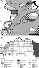 Figure 1
(A) Overview of the Latemar and neighboring Ladinian carbonate platforms and Upper Ladinian intrusions of the Dolomites. (B) East–west dike-perpendicular cross section across the Latemar platform (modified from Preto et al., 2011). The platform is subdivided into different lithozones (Egenhoff et al., 1999). Figure modified from Jacquemyn et al. (2014, and used with permission of Elsevier).
Figure 1
(A) Overview of the Latemar and neighboring Ladinian carbonate platforms and Upper Ladinian intrusions of the Dolomites. (B) East–west dike-perpendicular cross section across the Latemar platform (modified from Preto et al., 2011). The platform is subdivided into different lithozones (Egenhoff et al., 1999). Figure modified from Jacquemyn et al. (2014, and used with permission of Elsevier).
STUDY AIMS AND CONTEXT OF DIGITAL OUTCROP CHARACTERIZATION
The aims of this study are twofold. First, a suitable method is developed to derive three-dimensional (3-D) spatial lithology distribution from digital outcrop models (DOMs). Second, this approach is then applied to dolomite occurrences in the Latemar platform to understand the geometries and distribution of dolomite bodies in relation to igneous activity. A 3-D photorealistic DOM is created on which dolomite bodies can be defined more extensively, with more confidence and higher accuracy than in the field and can be validated by field observations. The challenge is to extract valuable quantitative geological information from such a model that describes the dolomite body geometry and distribution in 3-D at different scales.
Light detection and ranging (LIDAR) scanning is a well-established technique for generating high-accuracy, high-resolution DOMs. The use of LIDAR has become more widely used in reservoir outcrop analogue studies (Pringle et al., 2006; Martinsen et al., 2011) because it can generate DOMs on reservoir scale and provide data that can easily be implemented in geocellular reservoir models. However, quantification of geological information and subsequent interpretation obtained from DOMs both form challenges that are fairly new. Digital fieldwork on the DOM is required to gather data, and techniques have to be created or adapted to handle and interpret these new types of data (Kemeny et al., 2006; Martinsen et al., 2011; Monsen et al., 2011; Hodgetts, 2013).
Two types of LIDAR scanning projects can be distinguished (Jones et al., 2010). First, photo-realistic virtual outcrops are a digital copy of the real-world exposure, used for virtual field trips, safety reviews, and client meetings. Second, LIDAR scanning can be carried out for quantitative geological analysis. The latter is used to derive 3-D geometrical attributes for further (geospatial) analysis. In this study, LIDAR scanning is used for quantitative geological analysis of lithology distribution.
Geological data gathering from DOMs is mostly performed manually (or automatically if possible), either in the field or directly on the model. Integration of field observations into a DOM is mostly done in order to combine all gathered information geospatially, and it serves as calibration or starting point for geological simulations and realizations (Bellian et al., 2005; Verwer et al., 2009; Sharp et al., 2010; Gillespie et al., 2011; Preto et al., 2011; Amour et al., 2012; Van Noten et al., 2013). Observations can also be done directly on the DOM. This usually implies manual picking of XYZ points on the model in order to derive, for example, layering and platform geometry (Boro, 2012; Gramigna et al., 2013), faults, fractures, and slip vectors (Jones et al., 2009; Kurtzman et al., 2009; Rotevatn et al., 2009; Lapponi et al., 2011; Jacquemyn et al., 2012), vugs and karst cavities (Kurtzman et al., 2009; Labraña, 2011) or the geometry and distribution of sedimentary (Phelps et al., 2008; Fabuel-Perez et al., 2009) and diagenetic geobodies (Dewit et al., 2012). Several successful attempts are made for automated processing. Cyclostratigraphy was derived from LIDAR scans of limestone–marl alternations by Franceschi (2009) based on the intensity signal. For diagenetic studies in carbonates (e.g., dolomitization), the combination of hyperspectral imaging and LIDAR data is very promising (Kurz et al., 2012). Detailed variation of fault surface curvature is studied on LIDAR scans (Jones et al., 2009). A comparison between manual and semiautomatic fracture extraction (Wilson et al., 2011) suggests that automated methods mainly reveal well-exposed fracture sets and easily miss poorly exposed or smaller fracture traces. A review of possible quantitative data sets that can be obtained on LIDAR DOMs is presented in Tonon and Kottenstette (2007) and more recently in Jones et al. (2010). In most studies, 3-D geostatistics is the combination of a two-dimensional (2-D) horizontal and one-dimensional (1-D) vertical analysis (Kupfersberger and Deutsch, 1999).
None of the studies mentioned above present a method that can be applied to 3-D distribution of dolomite in the Latemar. Because the outcrop and the resulting lithology dataset is extensive in 3-D, dimension reduction to 2-D + 1-D is not possible. The approach developed here expands classical 2-D geostatistics to 3-D. Consequently, the concept of the 2-D variogram map is expanded to a 3-D variogram grid volume. Anisotropy analysis of the variogram grid aims to reveal the principal directions of dolomite occurrences and distribution in 3-D at multiple scales.
Spatial variation of dolomite occurrences is determined by the use of 3-D indicator variography computed from the 3-D lithology point cloud directly. Only limestone and dolomite are assessed, and because lithology is based on outcrop color, no further subdivisions can be made. In most studies, one dimension of an available 3-D dataset (often the vertical direction) is less pronounced, and thus, the spatial variation can be studied confidently in 2-D (e.g., Dewit et al., 2012). In this case, data reduction from 3-D to 2-D is not possible because the dataset is extensive in all three dimensions. Furthermore, 3-D variography in the literature often corresponds to the combination of 2-D bedding-parallel and 1-D vertical variography (Kupfersberger and Deutsch, 1999) and is not actually studied in 3-D as is done in this study. Although the approach in 3-D is similar to 2-D, mainly anisotropy detection differs significantly. Therefore, 2-D variogram maps and contour lines are replaced by their 3-D counterparts, respectively 3-D variogram grid volumes and contour surfaces. Furthermore, 2-D methods of anisotropy visualization and orientation determination are adapted to handle 3-D data.
Application of the 3-D variogram grid and subsequent anisotropy analysis on the Latemar lithology dataset shows that dolomite variation is clearly scale dependent. At a small scale (<200 m [656 ft]), dolomite bodies are elongated vertically or subhorizontally. Comparison of these principal directions to the average dike orientation indicates that dolomite bodies are extended parallel to the dikes. Stratigraphic control on the distribution of dolomite bodies becomes apparent at a larger scale (>200 m [656 ft]).
The results of the anisotropy analysis can directly be interpolated by indicator kriging in a reservoir model to allow visualization of the dolomite reservoir rock and can then serve for reservoir simulation. The resulting reservoir is a complex interfingering composite of horizontal and vertical dolomite bodies, with multiple connections to the underlying Contrin Formation.
GEOLOGICAL SETTING
Several Triassic carbonate platforms in the Dolomites, northern Italy, (Figure 1) are considered outcrop analogues for subsurface (dolomite) hydrocarbon reservoirs, for instance the Sella Group (Antonellini and Mollema, 2000), Pale di San Lucano (Blendinger and Meissner, 2006) and the Rosengarten or Catinaccio (Emmerich et al., 2009). Also in the Latemar, several aspects, such as platform geometry and fracturing, are covered in the literature as outcrop analogues.
The Latemar is a Middle Triassic isolated carbonate platform (Gaetani et al., 1981; Preto et al., 2011), located in the Dolomites (northern Italy). It is a steep-fronted (Marangon et al., 2011), mainly aggradational (Emmerich et al., 2005) to progradational (Preto et al., 2011) carbonate platform, which was deposited on top of a regional (mainly dolomitic) carbonate bank (Contrin Formation). The platform interior is subdivided into different lithozones (Goldhammer et al., 1987; Egenhoff et al., 1999), from bottom to top: Lower Platform Facies (LPF), Lower Teepee Facies (LTF), Lower Cyclic Facies (LCF), Middle Teepee Facies (MTF), Upper Cyclic Facies (UCF), and Upper Teepee Facies (UTF), respectively (Figure 1).
Carbonate production ceased during activity of the Predazzo volcanic complex in the late Ladinian (Bosellini, 1984). This activity consisted of an eruptive phase, which covered the Latemar and surrounding platforms with volcanic material, and subsequent emplacement of the Predazzo intrusion (Castellarin et al., 1982; Laurenzi and Visonà, 1996). Emplacement of the intrusion was coupled with emplacement of numerous north-northwest to south-southeast oriented dikes across the Latemar platform (Riva and Stefani, 2003). High-permeability brecciated zones along the dikes served as pathways for dolomitizing fluids that consequently caused (partial) dolomitization of the Latemar platform (Jacquemyn et al., 2014). Replacement dolomitization started during or shortly after dike emplacement. Mainly the stratigraphical lower half (LPF to MTF) is dolomitized, whereas the upper half does not contain large volumes of dolomite. An overview of the dolomitization mechanism and the importance of dikes in the dolomitization process is extensively covered in Jacquemyn et al. (2014).
A subjective non-quantitative description of the geometry of the dolomite bodies has been covered and revised by several authors. Earlier geometrical description of dolomite in the Latemar platform suggests a large mushroom-shaped dolomite body (Wilson et al., 1990). This model was revised by Carmichael et al. (2008) based on a more detailed description of the outcrops. A link was suggested between the presence of dikes and dolomite and dolomite geometry was described on single outcrop scale (>20 m [>65 ft]). However, both authors focused on the same stratigraphic interval, at the top of dolomite occurrences. The lower part that contains the most dolomite has not been studied in detail yet but is included in this study.
METHODOLOGY
LIDAR Acquisition and Model Building
The Latemar, and more specifically the Valsorda valley, possesses a difficult geometry for any scanning method because the majority of the dikes are easily eroded and form numerous incised valleys (Figure 2). Terrestrial LIDAR scanning would thus result in large areas of scanning shadow (Bonnaffe, 2007). A LIDAR helicopter-based scanning campaign in the Latemar was executed by Helimap System SA (
www.helimap.ch
). This is different from typical airborne scanning (vertical scanning) because the scanner is mounted to scan from oblique angles. Because the LIDAR scanner in the helicopter is moving, every incised valley is covered (at least partially) and scanning shadow is drastically reduced. The scanner used was a Riegl VQ-480 with a range of 1500 m (4921 ft), a rangefinder accuracy of 25 mm (0.98 in.) and a maximum angular resolution of 0.001°. The resulting point cloud resolution is on average 1.08 points per  of outcrop surface and covers an area of 2 by 2.5 km (1.55 mi). Detailed characteristics and resolution of the resulting 3-D geometry are listed in Table 1. Photographs were shot with a Hasselblad H4D camera (50 Mp resolution) mounted with a Hasselblad HC 35 mm f/3.5 lens (@f/6.8). The average scanning and photographing distance was approximately 350 m (1148 ft) resulting in a pixel size of 2–6 cm (0.78–2.36 in.). This resolution allows recognition of features (e.g., dolomite bodies) with an exposed surface area as small as
  (
( ). The resolution of the photographs is one order of magnitude higher than the merged point clouds. Projection of the photos on the LIDAR point cloud would, thus, result in a reduction of color resolution of the DOM. Because the Latemar DOM is used for lithology distribution based on color differences, high-resolution photographs are essential. In order to keep the highest possible resolution, the point cloud is converted to a triangulated mesh, and the photographs are draped on the resulting surface (Figure 3). Triangulation of the point cloud is executed in QTSculptor. Photograph draping is performed in RiScan Pro. For every photograph (700 in total), at least four control points (preferably 9–15) are picked manually on the photograph and on the blank, triangulated DOM. A fitting algorithm then calculates the photograph projection parameters and provides a fitting quality measure. Additional visual inspection is mandatory to ensure correct positioning of the photographs. The resulting DOM consists of a colored triangulated surface with a point resolution of approximately 1 m (3.28 ft) and a photo-pixel resolution of approximately 6 cm (19.68 ft). The digital terrain model (DTM) of the area is combined with the DOM to cover the whole Latemar platform. Although the spatial resolution of the DTM is lower than the DOM (Table 1), it is still sufficient to pick out the dike traces.
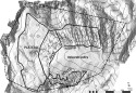 Figure 2
Overview of the digital outcrop model (DOM). The part of the DOM obtained by helicopter LIDAR scanning is indicated by solid black lines. It is subdivided into four zones that are smaller and easier to manipulate. The rest of the DOM is acquired from the digital terrain model (DTM). The outlines of the reservoir model are indicated by the dashed line. Sample sections are marked by their section number.
Figure 2
Overview of the digital outcrop model (DOM). The part of the DOM obtained by helicopter LIDAR scanning is indicated by solid black lines. It is subdivided into four zones that are smaller and easier to manipulate. The rest of the DOM is acquired from the digital terrain model (DTM). The outlines of the reservoir model are indicated by the dashed line. Sample sections are marked by their section number.
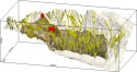 Figure 3
Northern half of the digital outcrop model (DOM). The textured part of the DOM is acquired by LIDAR scanning, whereas the white part is obtained from the digital terrain model. The traces of the mafic dikes are shown in yellow. The volcanic breccia pipes are marked in red. A color version of this figure is available in the online version of this paper.
Figure 3
Northern half of the digital outcrop model (DOM). The textured part of the DOM is acquired by LIDAR scanning, whereas the white part is obtained from the digital terrain model. The traces of the mafic dikes are shown in yellow. The volcanic breccia pipes are marked in red. A color version of this figure is available in the online version of this paper.

To assess the influence of topography on the geostatistical analysis, the DOM was subdivided into four zones (Figure 2). Three zones cover the steep rock walls surrounding the Valsorda valley (North, West, and South zone) and one is located on the Lastei di Valsorda plateau to the west of the Valsorda valley (Plateau zone). The latter, combined with the Path section in zone West (no. 10 in Figure 2), corresponds approximately to the area studied by Wilson et al. (1990) and Carmichael et al. (2008).
DOM Interpretation and Lithology Extraction
Lithology distribution in the Latemar is based on the manual selection of regions on the triangulated outcrop model, belonging to different lithologies. The centers of the selected triangles are used to represent the triangle lithology. Color differences between limestone and dolomite on the photograph are used for lithology recognition. Therefore, photograph quality (resolution, distortion, etc.) and color contrast are very important. Oblique projection of the photographs on the DOM was avoided in order to reduce picking uncertainties. Because the photographs are of higher resolution than the DOM, the resolution of the picked lithology is limited by the point cloud resolution. As a consequence, small-scale (<1 m [3.28 ft]) lithology variations (or lithology inaccuracies) will not be recorded.
Magmatic Dike Mapping
Numerous magmatic dikes crosscut the Latemar platform. The exact position and trajectory of these dikes are mapped on the 3-D DOM by selecting points on the DOM along their track (Figure 3). The inter-point distance is approximately 5 m (16 ft). Dikes can easily be recognized because they are more sensitive to weathering than carbonates and, thus, form steep, narrow gullies. The width of these gullies varies between 2 and 3 m (6.5 and 10 ft) and tens of meters. The mafic dike material is colored dark-brown to black and is clearly different from the gray and orange-brown carbonates. The weathered gullies are often filled by scree material that prevents observation of the rocks. Therefore, every gully is checked for the presence of magmatic dikes. If dike material is recognized, it is assumed the whole gully formed along a dike and was traced accordingly. In total, 385 mafic dikes are picked on the DOM.
The bottom of the Valsorda valley is composed of scree slopes and wood or bush areas. Consequently, no lithology can be mapped below the base of the exposed rock faces and no gullies can be traced. The dikes mapped on the southern and northern flanks of the Valsorda are probably connected, as they are also continuous on the plateau level from south to north. Due to branching and merging of the dikes, it is not possible to link dikes across the Valsorda valley.
Dolomite–Limestone Mapping
Dolomite and limestone occurrences are manually picked on the DOM based on the rock’s color. Dolomite generally exhibits an orange to brown color, whereas limestone is generally gray (Figure 4). However the difference between Fe-rich and Fe-poor dolomite, which was recognized in the diagenetical study (Jacquemyn et al., 2014), cannot be distinguished on the model. Rock samples and field observations are used for validation. Around 48% of the scanned surface is grass plain or scree slope that cannot be used for lithology partitioning.
 Figure 4
(A and B) Example of a photograph that is projected on the digital outcrop model on the northern flank of the Valsorda valley. A large dolomite body is located in the upper right corner of the photograph and model. Dolomite and limestone can be distinguished based on differences in rock color. (C and D) Two examples, at different scales, of clear dolomite versus limestone division are enlarged. Dolomite has an orange or brown patina, whereas limestone is mostly gray to white colored. The very high resolution of the photographs allows lithology distinction at meter scale (C).
Figure 4
(A and B) Example of a photograph that is projected on the digital outcrop model on the northern flank of the Valsorda valley. A large dolomite body is located in the upper right corner of the photograph and model. Dolomite and limestone can be distinguished based on differences in rock color. (C and D) Two examples, at different scales, of clear dolomite versus limestone division are enlarged. Dolomite has an orange or brown patina, whereas limestone is mostly gray to white colored. The very high resolution of the photographs allows lithology distinction at meter scale (C).
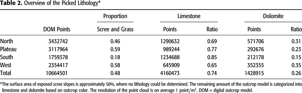
Locations where shadow or overexposed areas prohibit confident lithology recognition are disregarded, and thus, only well-exposed rock outcrops are used. This results in sets of georeferenced points of known lithology (Table 2) with an estimated resolution of one point per meter square of outcrop surface (Table 1). These points will be used to calculate the degree of dolomitization and derive its spatial distribution.
Geostatistics
The workflow and concepts of this approach will be introduced here. First, an omnidirectional semivariogram is calculated to determine if any spatial dependency is present in the lithology point cloud. Second, semivariogram grids are constructed that contain all possible directional semivariograms. These grids can reveal if lithology variation is isotropic (i.e., similar in all directions) or if lithology is more continuous or variable in specific directions. Directional dependence of lithology variation will result in anisotropy directions in the semivariogram grids. Third, along the observed anisotropy directions, predefined semivariogram models are fit to the experimental directional semivariograms.
Geostatistics are used to explore the spatial variability in datasets. In this case, the data are lithology points, being assigned a value of 0 or 1 for limestone and dolomite, respectively. The main geostatistical tool used here is the semivariogram. The semivariogram  is calculated as the half of the average squared difference between values of all point pairs, which are located a distance
  (lag) apart (Isaaks and Srivastava, 1989):
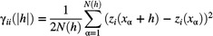
where  is the number of point pairs and
  and
and  are the values at the starting point and its corresponding end point, respectively (Figure 5).
Without any restrictions to the orientation of the point pairs, an omnidirectional semivariogram is calculated. To assess the spatial variability in specific directions, orientation constraints can be applied to the direction of distance vector  (Figure 6). Low semivariance indicates a low degree of variability (i.e., a high degree of similarity) between points, whereas higher semivariance indicates a higher degree of variability. Thus, increasing semivariance values with increasing distance indicate the presence of spatial correlation in the dataset.
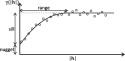 Figure 5
Example of an experimental semivariogram (circles) fitted by a spherical semivariogram model (solid line).
Figure 5
Example of an experimental semivariogram (circles) fitted by a spherical semivariogram model (solid line).
 Figure 6
Overview of (directional) semivariogram calculation parameters.
Figure 6
Overview of (directional) semivariogram calculation parameters.
The parameters that describe the spatial variation (variogram type, nugget, range, and sill) are determined by fitting positive definite semivariogram models to the experimental semivariogram. The number of point pairs,  , corresponding to the semivariogram values,
  , is used as a weight for the fitting algorithm.
Semivariograms are not only used for determining the variability in relation to inter-point distance. If the semivariogram parameters are different in function of direction, anisotropy is present. Variogram maps are typically utilized to detect anisotropy. Variogram maps are 2-D representations of directional semivariograms in all directions in a given plane, often horizontal or bedding parallel. These show the directional variability of the dataset within that plane. If certain directions exhibit variability over shorter or longer distances than others, anisotropy is geometric. If the sill values reached are dissimilar for different directions, anisotropy is zonal. Contouring of the semivariance values in a variogram map is commonly used for anisotropy detection (Sahin et al., 1998; Huysmans et al., 2008; Samal et al., 2011; Dewit et al., 2012; Possemiers et al., 2012, Franceschi et al., 2014).
In this study, the dataset is extensive in 3-D and cannot be reduced to a 2-D + 1-D case. Therefore, the 2-D variogram map concept is expanded into a 3-D variogram grid volume (Figure 7), which is a 3-D representation of all directional semivariograms in all directions. Therefore, the variogram grid shows 3-D directional variability. This forms a great improvement because it avoids calculating numerous variogram maps in many different directions, and it can provide a more accurate orientation of anisotropy because every direction is included in the grid and lacks the averaging that occurs when combining 2-D + 1-D. Analogous to the 2-D variogram map, 3-D contour surfaces of the semivariance can be calculated from the variogram grid and used to derive anisotropy. The amount of data points greatly exceeds the size of a typically gathered dataset, often only consisting of well data. Therefore, new algorithms are created to handle this amount of data. The Matlab code for variogram grid calculation is included in Jacquemyn (2013).
 Figure 7
Variogram grid of the complete lithology point cloud with a resolution of 5 m. Analogous to variogram maps, the center of the grid represents the starting point of all semivariograms. The semivariogram in a specific direction is then represented by a line crosscutting the variogram grid that starts in the center and follows this specific direction.
Figure 7
Variogram grid of the complete lithology point cloud with a resolution of 5 m. Analogous to variogram maps, the center of the grid represents the starting point of all semivariograms. The semivariogram in a specific direction is then represented by a line crosscutting the variogram grid that starts in the center and follows this specific direction.
Two-dimensional anisotropy is usually described by an ellipse, in 3-D this becomes an ellipsoid, controlled by three principal axes. The orientation of the long (R1), middle (R2), and short (R3) axes is derived by calculating the eigenvectors of the covariance matrix of the contour surface (similar to calculating a best-fit plane). Then directional experimental semivariograms are calculated along these three directions (R1–R3) to assess the spatial variability of the anisotropy ellipsoid. If different anisotropy directions exist for different semivariance contours, anisotropy is also scale dependent.
Experimental semivariograms are calculated from the dataset by using the aforementioned formula. However, for very large datasets (>100,000 data points), no software packages were available to handle this huge amount of data. Therefore, Matlab-scripts are created to calculate omnidirectional and directional semivariograms and variogram grids in an acceptable timeframe (Jacquemyn, 2013). Vector operations are used as much as possible to avoid successive loops over the enormous datasets. The computing time of the constructed algorithms is often more sensitive to the number of lags than to the number of data points. Additionally, the constraints to obtain directional semivariograms greatly improve calculation times. Averaged point pair calculation time for 700,000 points over 600 lags is approximately 1.6 million point pairs per second. Because no software packages are available to straightforwardly assess the 3-D variability, a Matlab script was created for the calculation and export of semivariogram grids. The variogram grid calculation time is, analogous to semivariogram calculation, more sensitive to the grid density (lag distance) than to the number of input points. The grid is exported as a uniform rectilinear VTK grid (Schroeder et al., 2006), which can easily be visualized and analyzed by most 3-D software packages.
RESULTS: LITHOLOGY DISTRIBUTION
The distribution of replacement dolomitization is assessed by acquiring lithology information through manual interpretation of a photorealistic 3-D DOM at high accuracy with high resolution. The 3-D DOMs obtained by LIDAR scanning provide the accuracy and detail, at large enough scale, necessary to achieve a reliable and, yet, extensive quantitative 3-D lithology dataset. The resulting lithology point cloud can then be investigated statistically to describe the spatial distribution of dolomite occurrences. In addition to carbonates, dike occurrences can also be picked on the DOM. From these point picks, dike orientation and spacing can accurately be determined.
Magmatic Dike Mapping
The exact position and trajectory of the dikes are mapped on the 3-D DOM by selecting points on the DOM along their track (Figure 3). The orientation of the dikes is estimated by calculating the best-fit plane, using orthogonal regression (Fernández, 2005; Jones et al., 2009).
The orientation results are displayed in Figure 8. The majority of the dikes are subvertical (∼87°) and dominantly oriented north-northwest. The rose diagram of the strike values (Figure 8) confirms that the majority of the dikes’ strike is close to 325°. Very few dikes are oriented more than 20° apart from 325°.
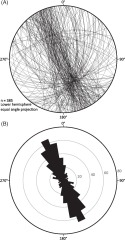 Figure 8
The orientation of all dikes is calculated by fitting a plane to the dike traces. (A) Equal angle lower hemisphere stereographic projections of all dikes. (B) Bi-directional rose diagram of the strike of all dikes. The main strike direction is approximately 325°.
Figure 8
The orientation of all dikes is calculated by fitting a plane to the dike traces. (A) Equal angle lower hemisphere stereographic projections of all dikes. (B) Bi-directional rose diagram of the strike of all dikes. The main strike direction is approximately 325°.
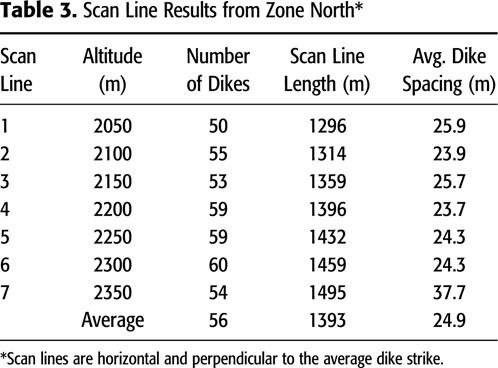
Dikes are closely spaced. In zone North, dike occurrences are counted along horizontal scan lines perpendicular to the dikes’ average azimuth (analogous to mechanical stratigraphy scan lines). Seven scan lines are calculated, spaced 50 m (164 ft) vertically from 2050 to 2350 m (6725 to 7709 ft) altitude (Table 3). The average number of dikes encountered and scan line length are 56 dikes and 1393 m (4570 ft), respectively. Both values combined results in an average spacing of 27.6 m (90.55 ft). Although branching is observed in several dikes, the average dike spacing remains constant over the studied interval. Systematic dike thickness measurements are not available; however the average dike thickness is estimated to be at least 2 m (6.5 ft) based on field observations. Consequently 56 dikes over on average 1400 m-long (4593 ft) scan lines, correspond to a cumulative thickness of 112 m (367 ft) of dikes, which corresponds to a minimum of 8.0% of magmatic material in the total rock volume.
Carbonate Distribution Acquisition
Manual detection of lithology on the DOM results in a lithology point cloud of more than 5.5 million points (Table 2). Approximately 48% of the original DOM was covered with scree slopes and grass areas and cannot be used for lithology detection. The lithology point cloud contains more than 4.1 million points that represent limestone and 1.4 million for dolomite (Figure 9). On average, 26% of the scanned outcrops on the Latemar and in the Valsorda valley consist of dolomite. Some variation in dolomite distribution exists between the different zones, from 15% in zone South to 35% in zone West. Most of the dolomite occurs in the lowest part, in or just above the Contrin Formation.
 Figure 9
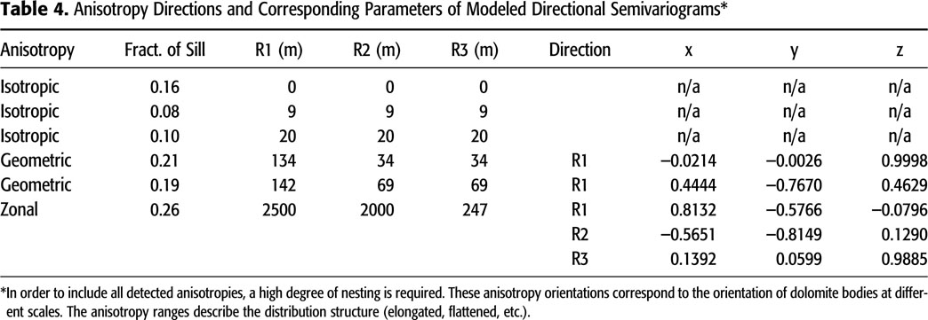
Map view of the DOM, colored according to carbonate lithology. The areas that could not be characterized (scree, grass, etc.) are uncolored.
Figure 9
Map view of the DOM, colored according to carbonate lithology. The areas that could not be characterized (scree, grass, etc.) are uncolored.
The vertical proportion curve (VPC) reflects the ratio of dolomite versus limestone in function of stratigraphic (vertical) height above the base of the Contrin Formation (Figure 10). Corresponding to field observations, the Contrin Formation is almost completely dolomitized. The low percentage of limestone might be the result of incorrect delineation of the top of the Contrin Formation, or it might be caused by displacement along normal faults of blocks of the overlying LPF. The dolomite percentage in the lower half of the LPF drops radically from 90% to approximately 23%. The height interval along which the dolomite percentage decreases is roughly 200 m (656 ft). This is probably caused by the dolomite bodies that rise from the Contrin Formation into the LPF. Some of these bodies end within 150 m (492 ft) above the Contrin Formation, whereas others reach much higher and form vertical dolomite bodies. From halfway up in the LPF up to the top of the LCF, the dolomitization percentage is roughly constant around 23%. In the MTF, dolomitization decreases to zero over a height interval of 100 m (328 ft). No lithology points are available from the UCF and UTF, but based on field observations and literature data, these are considered devoid from large amounts of replacement dolomite.
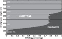 Figure 10
Vertical proportion curve of lithology. Only the carbonate fraction is considered in this plot, and the magmatic bodies are disregarded. The Contrin Formation is almost completely dolomitized, and the UCF and UTF are basically free from replacement dolomite. The lower part of the LPF shows a strong decrease in dolomite–limestone ratio and stagnates around 23%. This value is maintained up to the top of the LCF. In the MTF, the dolomite percentage drops to zero.
Figure 10
Vertical proportion curve of lithology. Only the carbonate fraction is considered in this plot, and the magmatic bodies are disregarded. The Contrin Formation is almost completely dolomitized, and the UCF and UTF are basically free from replacement dolomite. The lower part of the LPF shows a strong decrease in dolomite–limestone ratio and stagnates around 23%. This value is maintained up to the top of the LCF. In the MTF, the dolomite percentage drops to zero.
Geostatistics
The resulting parameters of the semivariogram models, complemented by the anisotropy directions, provide a mathematical description of the dolomite distribution that will be used for subsequent reservoir model construction.
Omnidirectional Semivariogram
To estimate an overall distance range and degree at which limestone–dolomite variations occur, an omnidirectional experimental indicator semivariogram is calculated for the whole dataset (circles in Figure 11). The experimental semivariogram increases gradually from 0.030 (nugget) to a total sill of 0.186 at a distance of approximately 1200 m (3937 ft). This indicates that limestone–dolomite presence is spatially autocorrelated up to distances of 1200 m (3937 ft).
 Figure 11
Experimental omnidirectional semivariograms of the complete limestone–dolomite dataset (circles) and the complete dataset except the points belonging to the Contrin Formation (triangles). Their curves are relatively similar up to 400 m (1312 ft), at larger distances an average difference of 0.015 exists between both curves. Nested semivariogram models are fit to both experimental semivariograms (solid lines).
Figure 11
Experimental omnidirectional semivariograms of the complete limestone–dolomite dataset (circles) and the complete dataset except the points belonging to the Contrin Formation (triangles). Their curves are relatively similar up to 400 m (1312 ft), at larger distances an average difference of 0.015 exists between both curves. Nested semivariogram models are fit to both experimental semivariograms (solid lines).
Therefore, we conclude that dolomite is not distributed randomly, and further directional analysis is useful. Starting at a distance of approximately 1300 m (4265 ft), the reliability of the experimental semivariogram starts to decrease significantly because the number of available point pairs starts to decrease. Therefore, values at distances exceeding 1300 m (4265 ft) are disregarded. However, the most significant change in semivariance occurs in a distance range from 0 to 500 m (0 to 1640 ft). Around a distance of 400 m (1312 ft), semivariance increase is reduced dramatically. This is probably caused by the lack of vertical point pairs at longer distances because the vertical extent of the point cloud is roughly 500 m (1640 ft). Because the vertical extent of the lithology dataset is three times smaller than the horizontal extent, preferably directional semivariograms should be used to describe the 3-D spatial variability. The orientations that best describe the limestone–dolomite variations are determined by an anisotropy analysis.
Additionally an omnidirectional semivariogram is calculated for the dataset without the points belonging to the Contrin Formation (Figure 11, triangles) to assess the influence of this dolomitic bank. Generally, this curve follows the overall semivariogram at distances up to approximately 400 m (1312 ft). For distances exceeding 400 m (1312 ft), the semivariogram of the cropped dataset stagnates and is on average 0.015 lower than the overall semivariogram. The largest contribution of the Contrin Formation to the overall spatial variability is, thus, present in the range up to 400 m (1312 ft) and, based on the extent of the dataset, probably mainly in (sub)vertical directions. Additionally, the calculated ranges are slightly shorter than the ranges for the complete dataset. Because several dolomite bodies rise up from the Contrin Formation, the complete point cloud (including Contrin Formation) will be used for further analysis in order to include its influence on the dolomite distribution. With the use of a VPC, it is guaranteed that during kriging interpolation the Contrin Formation contains only dolomite.
Dolomite Anisotropy Detection
Dolomite distribution in the Latemar platform was previously described in distinct shapes (vertical pipe, horizontal bodies, and fingers). However, these descriptors are subjective terms. Objective description of the dolomite distribution is advisable. As shown above, directional variography is ideal to describe spatial limestone–dolomite variation geostatistically. The principal directions that best describe this lithology variation can be determined by a 3-D anisotropy analysis.
Anisotropy is present in the dataset when its pattern of spatial variability changes with direction. In that case, descriptors of spatial relationships, such as semivariogram ranges and sills, are different in different directions. Variogram grids are calculated to determine the 3-D semivariance of lithology in all possible directions and thus reveal and quantify anisotropy. The principal directions (and corresponding semivariogram parameters) of lithology variations are an indication of dolomite body geometry and dolomite body distribution.
Because the extent and resolution of the lithology point cloud is too large to be covered completely, at maximum variogram grid resolution, a subdivision is made between small-scale (<200 m [<656 ft]) and large-scale features (>200 m [>656 ft]), using variogram grids with cell resolutions of 5 and 20 m (16 and 65 ft), respectively. The 200 m (656 ft) threshold between small- and large-scale grid size is determined arbitrarily, based on calculation times and the variation in the omnidirectional variogram, indicating that a large part of the variation occurs within a range of 200 m (656 ft). Additionally, this corresponds to the visually estimated average dolomite body size, observed in outcrop.
Similar to 2-D anisotropy analysis by contour lines on variogram maps (e.g., Lombardi and Voltattorni, 2010), 3-D semivariance isocontour surfaces can reveal the presence of anisotropy and determine its principal directions. For low semivariance values (≤0.08), the contours result in spheres, and thus, lithology variation is isotropic (no directional influence). Figure 12 shows 3-D contour surfaces at 0.09 semivariance of variogram grids of  (
( ) with a 5 m (16 ft) cell size for all data combined, as well as every zone separately. The contour surface for all data resembles two prolate ellipsoids (rather than tri-axial ellipsoids), one subvertical and one subhorizontal. These anisotropy ellipsoids each represent an anisotropy direction and crosscut each other at approximately 63°. The long axes (R1) of both ellipsoids represent directions of more gradual increase in semivariance with distance compared to other directions and, thus, the directions of maximal spatial continuity. Alternatively, these directions correspond to the orientation of dolomite bodies (dolomite
  of continuous lithology). Therefore, we conclude that on a small scale (<200 m [<656 ft]) dolomite bodies have one main axis that is aligned either vertically or horizontally. The prolate geometry of the ellipsoids suggests the maximum variability is isotropic perpendicular to the long axes. The common plane of both ellipsoids is calculated by fitting a plane to the contour surface. The long axes (R1) of the anisotropy ellipsoids are located in this plane. The normal direction to the fitted plane will be used for determining the short ranges of both anisotropy ellipsoids during the semivariogram modeling step. Ellipsoid orientation values are listed in Table 4. The strike orientation of this common plane, along which dolomite bodies are aligned, is 322°, which is only 3° difference from the average orientation of the magmatic dikes.
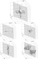 Figure 12
Three-dimensional contour surfaces at 0.09 of the variogram grids for the entire dataset and every zone separately. Orientation of all boxes is identical. The gray plane represents the best fit plane to the contour at 0.09 of all data. The subvertical and subhorizontal anisotropy is clearly visible for all data combined. For the separate zones, outcrop orientation has an important control on the contours. For example, the contour of the Plateau zone lacks the subvertical anisotropy. This can be explained by the fact that the topography of this zone is rather flat, and thus, very few vertically oriented point pairs are available. In every grid, it can be observed that anisotropy contours occur along the fitted plane.
Figure 12
Three-dimensional contour surfaces at 0.09 of the variogram grids for the entire dataset and every zone separately. Orientation of all boxes is identical. The gray plane represents the best fit plane to the contour at 0.09 of all data. The subvertical and subhorizontal anisotropy is clearly visible for all data combined. For the separate zones, outcrop orientation has an important control on the contours. For example, the contour of the Plateau zone lacks the subvertical anisotropy. This can be explained by the fact that the topography of this zone is rather flat, and thus, very few vertically oriented point pairs are available. In every grid, it can be observed that anisotropy contours occur along the fitted plane.
To verify whether the acquired anisotropy ellipsoids are valid for subsets of the lithology point cloud, the anisotropy analysis is repeated for each of the four zones (Figure 2) separately. Both anisotropy ellipsoids do not occur in every variogram grid of the individual zones (Figure 12). The contour surface of the Plateau zone represents only a subhorizontal ellipsoid. Due to the rather horizontal outcrop topography of this zone, too few vertical point pairs can be assessed to confidently calculate semivariance in a vertical direction, and thus, vertical variability cannot be considered based on this part of the dataset alone. The same reasoning explains why the subhorizontal anisotropy is not present in the variogram grid of zone West. Few point pairs along a N30E direction exist in this part of the dataset. In zones North and South, both the subvertical and subhorizontal anisotropy directions can be observed. For zone South, both anisotropies appear to be connected in the upper-north quadrant. This is, however, the quadrant for which the fewest point pairs exist because the general direction of this zone is dipping north. A similar phenomenon is observed in zone North, where the subhorizontal anisotropy contour surface widens toward the quadrant with the least point pairs (upper-south). These effects are, therefore, considered to be caused by outcrop topography and not by lithology variability. The subvertical and subhorizontal anisotropy directions are detected in every zone and are, thus, valid for the whole dataset and its subsets.
Similar to small-scale variogram grids, large-scale variogram grids are used to determine the parameters of large-scale lithology variation. Therefore, a large variogram grid of  (
( ) with a grid cell size of 20 m (65 ft) is calculated from the complete lithology point cloud (Figure 7). Figure 13 shows the contour surface at semivariance 0.18. The contour surface exists of two parts that are not connected. This indicates that sample continuity in between both parts of the contour surface is much larger and does not reach the same semivariance value as perpendicular to the surface, and thus, zonal anisotropy is present.
 Figure 13
Contour surface (green) of a large-scale variogram grid at 0.18 semivariance. The best-fit plane to the contour surface is marked in blue and is slightly dipping to the northeast. The anisotropy orientation is equal to bedding. The small-scale anisotropy contour surface is added in red for comparison (center of the picture). A color version of this figure can be seen in the online version of this paper.
Figure 13
Contour surface (green) of a large-scale variogram grid at 0.18 semivariance. The best-fit plane to the contour surface is marked in blue and is slightly dipping to the northeast. The anisotropy orientation is equal to bedding. The small-scale anisotropy contour surface is added in red for comparison (center of the picture). A color version of this figure can be seen in the online version of this paper.
The orientation of anisotropy is determined by calculating a best-fit plane to the contour surface. The plane-normal represents the shortest axis (R3) of the anisotropy ellipsoid and, thus, the direction of highest lithology variability. Dip and dip direction values of this plane are 8.7 and 66.7°, respectively, and are, thus, parallel to bedding (Preto et al., 2011). The remaining axes that describe the large-scale anisotropy ellipsoid are located along the best-fit plane. This planes holds the directions of maximum lithology continuity. Contouring of the 2-D variogram map, parallel to this plane, shows that the middle and long axes of the anisotropy ellipsoid are oriented parallel to southwest–northeast and northwest–southeast, respectively. Because anisotropy is present within this plane, anisotropy at this large scale is modeled as a tri-axial ellipsoid, and two additional principal axes were determined. Anisotropy orientation directions are listed in Table 4. The large-scale anisotropy cannot be assessed separately for individual zones, analogous to the small-scale anisotropies, because these zones are not large enough, so the number of point pairs at long distances would be insufficient.
Directional Semivariogram Modeling
Based on semivariance contouring, three anisotropy ellipsoids are recognized at different scales. The two small-scale anisotropies correspond to lithology variation and geometry at dolomite body scale, whereas the large-scale anisotropy corresponds to dolomite body distribution. The geostatistical parameters, such as sills and ranges, corresponding to the different anisotropies, are determined along the principal axes of the anisotropy ellipsoids. These parameters describe the degree and distance of lithology variation in these principal directions and can be applied directly for reservoir model construction.
For all three detected anisotropies, semivariograms are modeled along their principal axes. The threshold and cone length of the directional constraints are set at 2× lag spacing and 5× threshold, respectively, for all directional semivariograms. The lag spacing and maximum distances used are determined by the anisotropy scale.
The small-scale anisotropy is assessed by calculating three experimental directional semivariograms with a lag spacing of 2 m (6 ft) (100 lags). These are calculated along the long axes of the ellipsoids of both small-scale anisotropies and perpendicular to their common plane (Figure 12). Because calculation time increases drastically with the number of lags, the maximum distance is limited to 200 m (656 ft). Because larger scale structures are present, the experimental semivariogram does not reach the total sill in the depicted range. The parameters of the large-scale anisotropy are determined by three experimental directional semivariograms with a lag spacing of 5 m (16 ft) (200 lags) along the corresponding principal directions. It should be noted that all anisotropies also have an influence on each other. Therefore, the resulting overall model has to include a degree of nesting of at least the number of anisotropies. The resulting experimental semivariograms along these six directions (three small scale and three large scale) are then used for fitting semivariogram models with nesting up to 4°. The number of point pairs are used as weights to improve reliability of the resulting models. The geostatistical parameters (range and sill) are then derived from the different nested semivariograms (Table 4).
The modeled semivariograms exist of several nested spherical semivariograms (including nugget). Consequently, a rather complex model is required to objectively describe dolomite distribution in the Latemar. This complexity is needed to include the variation at different scales and variation in distinctly different orientations.
The geostatistical approach to the lithology dataset describes the spatial variability of dolomite occurrence. The obtained semivariogram parameters and corresponding anisotropy direction will be applied to the dataset itself to interpolate lithology in the reservoir model. However, these characteristics can also be directly applied to any dataset of georeferenced lithology points for which similar dolomitization processes are identified or suspected, or similar relationships are observed in relation to, for example, magmatic dikes.
Reservoir Modeling
Carbonate and dikes are mapped in the field as well as on the 3-D DOM. Spatial distribution of dolomite versus limestone is geostatistically investigated. Consecutively, this lithology information (location + variography parameters) is implemented into the reservoir grid model by allocating a lithology value to every cell in correspondence to the derived lithology statistics. Discrete values are assigned to the various lithology classes.
Dolomite distribution is extensively characterized by applying geostatistics to the lithology dataset. For reservoir model construction, kriging interpolation of the lithology dataset is performed to assign lithology values to every grid cell of the reservoir model. The required input for kriging is the defined anisotropy directions, the parameters of the fitted semivariogram models, and the VPC.
The whole lithology point cloud is inserted into a reservoir model. A rectilinear cornerpoint grid with 335 × 445 × 130 cells, with a size of 8 × 8 × 8 m (26 × 26 × 26 ft), is used to cover the whole study area. Lithology values (0 and 1 for limestone and dolomite, respectively) from the point cloud are assigned to their corresponding grid cells. At this stage 120,740 out of 13,401,461 cells (0.9%) are appointed a lithology value. The remaining empty cells will be assigned a lithology based on the geostatistical analysis described earlier. As suggested by Amour et al. (2012), sequential indicator simulation (SIS) is recommended for modeling complex geological heterogeneity and geometry. Therefore, all remaining cells are interpolated by applying simple indicator kriging with SIS based on the geostatistical parameters listed in Table 4. The kriging interpolation is constrained by the known lithology point cloud and the VPC of dolomite occurrence (Figure 10). The resulting dolomite distribution is shown in Figures 14 and 15.
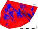 Figure 14
Horizontal cross section through the reservoir model at the top of LPF after carbonate lithology kriging and emplacement of igneous rocks, showing the limestone and dolomite distribution. The outline of the Valsorda valley is indicated by a white dashed line. The mafic dikes are marked by light gray lines. The lack of dikes in the middle of the model is the result of the lack of information on the dike traces in the Valsorda.
Figure 14
Horizontal cross section through the reservoir model at the top of LPF after carbonate lithology kriging and emplacement of igneous rocks, showing the limestone and dolomite distribution. The outline of the Valsorda valley is indicated by a white dashed line. The mafic dikes are marked by light gray lines. The lack of dikes in the middle of the model is the result of the lack of information on the dike traces in the Valsorda.
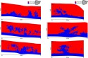 Figure 15
Dike-perpendicular (A–C) and dike-parallel (D–F) vertical cross sections through the reservoir model. The Contrin Formation, at the base of the model, is completely dolomitized. Similarly, the top of the model consists of 100% limestone, based on field observations, which are not interpolated. This results in sharp upper boundaries of the dolomite bodies. (A) Vertical dolomite chimneys can be observed that rise up from the Contrin Formation. (B) Not all dolomite bodies are connected directly vertically to the Contrin Formation but have a horizontal connection to a dolomite pipe. Isolated dolomite bodies only account for 10% of the total dolomite volume. (C) Not only do vertical dolomite pipe rise up high into the Latemar Formation, wide triangular dolomite bodies also exist. (D and E) Parallel to the dikes, dolomite pipes are not always vertical, but large dolomite pipes are always rooted in the Contrin Formation. (F) Sub-vertical dolomite pipe with horizontal dolomite bodies.
Figure 15
Dike-perpendicular (A–C) and dike-parallel (D–F) vertical cross sections through the reservoir model. The Contrin Formation, at the base of the model, is completely dolomitized. Similarly, the top of the model consists of 100% limestone, based on field observations, which are not interpolated. This results in sharp upper boundaries of the dolomite bodies. (A) Vertical dolomite chimneys can be observed that rise up from the Contrin Formation. (B) Not all dolomite bodies are connected directly vertically to the Contrin Formation but have a horizontal connection to a dolomite pipe. Isolated dolomite bodies only account for 10% of the total dolomite volume. (C) Not only do vertical dolomite pipe rise up high into the Latemar Formation, wide triangular dolomite bodies also exist. (D and E) Parallel to the dikes, dolomite pipes are not always vertical, but large dolomite pipes are always rooted in the Contrin Formation. (F) Sub-vertical dolomite pipe with horizontal dolomite bodies.
Because the average grid cell size of the complete model is 8 × 8 × 8 m (26 × 26 × 26 ft), the nested semivariogram with the smallest range (9 m [29 ft]) is omitted to increase computation performance, and its contribution is added to the nugget effect. If included, the effect of this variogram would be minimal because its range is very close to the average cell size. In order to interpolate the finer grids, this sub-variogram cannot be disregarded.
The resulting model (Figure 14) shows a complex composite of interfingering vertical and horizontal dolomite bodies. Alignment to the dikes can clearly be observed. In vertical cross sections (Figure 15), the connection between the Contrin Formation and vertical dolomite bodies can be observed. The latter often have a wide base at the contact and become narrower higher up in the stratigraphy. In dike-perpendicular cross sections, several isolated dolomite bodies are present, however, in dike-parallel sections these are mostly connected to other (vertical and horizontal) dolomite bodies.
DISCUSSION
Many different approaches exist considering the processing of geospatial data in the function of the goals (Amour et al., 2012). In many studies, sedimentary evolution, lateral facies variation (Pranter et al., 2005; Budd et al., 2006; Palermo et al., 2010), or platform geometry (Phelps et al., 2008; Verwer et al., 2009) is investigated. Often, the distinction between horizontal (or bedding parallel) and vertical (layer stacking) is well defined and a 3-D problem can be reduced to a combination of 2-D horizontal and 1-D vertical variography (Kupfersberger and Deutsch, 1999; Willis and White, 2000; Qi et al., 2007). Some studies calculate the statistical description of geobody geometry in terms of parameters such as length, width, and height (Qi et al., 2007; Fabuel-Perez et al., 2009) or implement predefined geometries (Mikes and Geel, 2006). However, only a few studies deal with dolomite bodies, stratabound (Koehrer et al., 2010) or fault-controlled (Lapponi et al., 2011; Dewit et al., 2012).
Because dolomitization of the Latemar platform is not limited to lateral or stratigraphical variation or geometrically well-defined geo-bodies, none of the approaches listed previously can be directly applied. Dewit et al. (2012) have successfully applied a 2-D variography geostatistics on hydrothermal dolomites in northern Spain. Anisotropy analysis of the dolomite bodies indicated a clear relationship between their orientation and the fault system. For this case, 2-D geostatistical analysis is adapted to 3-D. The approach followed is often not only dictated by the goals but also by data availability. In very few cases, exceptional 3-D outcrop geometry, combined with high-resolution lithology (or facies) information is available, which is a prerequisite for actual 3-D variography. As is suggested by variography of the subsets, a complete 3-D outcrop is required. Variography on one or two (oriented) subsets alone would yield significantly different results.
Three-dimensional variography reveals that at least three anisotropy directions are present in the distribution of the studied carbonates. These anisotropy directions cover lithology variations at a different scale. The small-scale anisotropy directions are oriented roughly horizontally and vertically and have a range smaller than 150 m (492 ft) along their major principal axes (R1). These anisotropies are considered to be governed by dolomite body geometry. Dolomite bodies described in this study, as well as described by Carmichael et al. (2008), are mainly vertical bodies (pipes) and horizontal extensions of these pipes (layer-parallel fingers). The vertical anisotropy direction is a manifestation of the vertical pipe-like bodies. Correspondingly, the subhorizontal anisotropy is the representation of horizontal dolomite bodies. Both anisotropies (and thus lithology) are oriented along a common, subvertical plane (Figure 12). The orientation of this plane is nearly parallel to the main orientation of the dikes (Figure 16). Therefore, the outlines of dolomite bodies are aligned along the mafic dikes, either vertically or horizontally. This confirms the dike control on fluid flow that exists between the dikes and hydrothermal dolomitization (Jacquemyn et al., 2014). A spatial relationship between dikes and dolomite bodies was already suggested in the literature (Carmichael et al., 2008), however this could not be checked quantitatively.
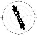 Figure 16
Rose diagram of the dike orientation data (black) compared to the common plane of both small-scale anisotropy orientations (white arrow). The difference between the main dike orientation and the shared anisotropy plane is less than 3°.
Figure 16
Rose diagram of the dike orientation data (black) compared to the common plane of both small-scale anisotropy orientations (white arrow). The difference between the main dike orientation and the shared anisotropy plane is less than 3°.
The large-scale anisotropy corresponds to dolomite body distribution rather than individual dolomite body geometry. This anisotropy is subhorizontal, slightly dipping to the northeast. The dip (8°) and dip direction correspond closely to the orientation of the growth wedge observed in the central portion of the Plateau zone (Preto et al., 2011). This indicates that dolomite body occurrence is probably governed (at least partially) by sedimentary facies. An additional indication for facies dependency is the sudden drop of the dolomite versus the limestone ratio in the MTF (Figure 10).
The calculated VPC (Figure 10) is contradictory with the curve constructed by Carmichael et al. (2008) that is based on field mapping along six traverses with a total length of 9.7 km (6 mi). Because only one of these traverses crosscuts the LPF, the coverage of this facies is limited. Hence, this is the facies where results are clearly different. In this study, the lithology dataset is evenly distributed over the complete studied interval and can, therefore, be considered more accurate. The constructed VPC is also used to constrain lithology kriging interpolation.
Variography revealed an important association between dolomite occurrence and mafic dikes. Cross sections (Figure 15) through the reservoir model show the dolomite distribution parallel and perpendicular to the main dike direction. Several vertical pipe-shaped dolomite bodies are present, rising above the Contrin Formation. The presence of one of these pipes at the southwest end of the Valsorda was already described by several authors (Wilson et al., 1990; Carmichael et al., 2008). The outline and incidence of the dolomite pipes are similar to the diagenetic chimneys shown by Esteban et al. (2005) that are also associated with fractures and form chimney-like geobodies. The geometry of the dolomite pipes is much like what is described by Lapponi et al. (2011) in the Zagros Mountains in Iran. Correspondingly, most dolomite bodies in the Latemar are also rooted in a massive volume of dolomite (Contrin Formation). Pipes are generally more tabular than circular as the term pipe suggests (with a shorter direction perpendicular to main dike orientation).
However, not all pipes formed vertical structures because some are inclined in cross sections parallel to the main dike orientation. No preferential inclination direction (north or south) is observed. Inclination is not controlled by sampling geometry, i.e., constraints imposed by the presence of the Valsorda valley because inclination also occurs in vertically stacked bodies, whereas the inclined flanks of the Valsorda are not vertically stacked. Possibly, diagonal dolomite bodies are the result of superposition of both small-scale anisotropies (horizontal and vertical).
Several dolomite bodies rise up from the Contrin Formation that do not exhibit a pipe-like geometry. In contrast, these have a triangular or pyramidal vertical outline that is wide at the contact with the Contrin Formation and becomes narrower with increasing height. These are probably preserved in an early stage of dolomite pipe development. In this study, many isolated bodies are observed in the field and can be quantified in the reservoir model. Large, isolated dolomite bodies (at least one dimension exceeding 50 m [64 ft]) are often horizontally aligned and account for approximately 10% of the dolomite volume above the Contrin Formation. Because of the interfingering of different dolomite bodies in three dimensions, these isolated bodies are probably connected to other dolomite bodies.
The spacing between different dikes could play an important role on the width of the dolomite bodies and their spacing. Because the dike-spacing is constant in this study, the control distance between different dolomite bodies cannot be derived from this dataset alone. Therefore, additional case studies are needed with different distribution of the dikes, such as in the nearby Marmolada platform.
The combination of the small-scale vertical and horizontal anisotropies results in vertical dolomite bodies (pipes), in some cases with horizontal dolomite bodies attached. These horizontal dolomite extensions do not only occur in the LTF and LCF (Carmichael et al., 2008) but also lower in the LPF (Figures 10 and 15). Furthermore, these horizontal extensions can form a connection between vertical dolomite bodies. This combination results in a complex, interconnected pattern of very porous dolomite. Other features facilitating or inhibiting flow are discussed in Jacuemyn et al. (2014).
Application of 3-D variography is very useful to understand the spatial variation of lithology and can easily be integrated with reservoir modeling workflows. The results of this work or other applications of this approach can be directly implemented to analogous reservoirs by applying the spatial relationships uncovered here (Table 4) on available conditioning data from the subsurface, such as well data or seismic interpretation. However, some disadvantages exist, e.g., for reliable results a data-rich 3-D scenario is required to calculate the spatial relationships, such as DOMs. For example, analysis of 3-D seismic data that has been inverted for lithology could benefit from this technique for the construction of reservoir models. Applications are not limited to spatial lithology variation but can be extended to all spatial 3-D data on a wide range of scales (e.g., porosity variation in rock samples). The next promising step in 3-D analysis would be 3-D multiple points statistics that could result in more accurate interpolation.
CONCLUSIONS
Dolomitization in carbonate platforms affected by igneous activity has become more interesting recently for oil and gas exploration. Until now, very little has been known about the possible distribution and geometry of hydrothermal dolomite in this type of play. The Latemar platform presents a unique reservoir analogue for a carbonate platform that is crosscut by mafic dikes and is affected by dolomitization. The 3-D organization of the rock exposures form a perfect location to determine the geometry and distribution of dolomite bodies at multiple scales.
Lithology is derived from a 3-D photorealistic DOM. The DOMs provide a valuable tool for geological and reservoir analogue studies. An important challenge exists in extracting meaningful information from these DOMs. Therefore, a new approach was created to assess the distribution of lithology in true 3-D (not 2-D horizontal + 1-D vertical). Classical geostatistical concepts (2-D variogram map and anisotropy detection) are expanded to the 3-D variogram grid and resulting 3-D contour surface to represent anisotropy and, thus, provide insight into dolomite body distribution. An additional advantage lies in the fact that the results of this 3-D geostatistical application on outcrop analogues can immediately be implemented for constructing reservoir models.
This novel approach is successfully applied to the dolomite occurrences in the Latemar platform. Previous descriptions of distribution and geometry of the dolomite bodies depended on generic descriptions. The complex outcrop morphology requires a quantitative approach. The results presented here are the first 3-D description of dolomite bodies in a carbonate platform affected by igneous activity. The small scale (<200 m [656 ft]) distribution of dolomite shows that dolomite bodies are elongated, vertically or subhorizontally, and are preferentially oriented parallel to the main dike orientation (N30W). This confirms the genetic link that exists in the Latemar between dolomite and dikes. The large-scale (200–1600 m [656–5249 ft]) dolomite distribution highlights the control of stratigraphy on dolomite body distribution.
REFERENCES CITED
Al-Awadi, M., W. J. Clark, W. R. Moore, M. Herron, T. Zhang, W. Zhao, N. Hurley, D. Kho, B. Montaron, and F. Sadooni, 2009, Dolomite: Perspectives on a perplexing mineral: Oilfield Review, v. 21, p. 32–45.
Amour, F., M. Mutti, N. Christ, A. Immenhauser, S. M. Agar, G. S. Benson, S. Tomás, R. Alway, and L. Kabiri, 2012, Capturing and modelling metre-scale spatial facies heterogeneity in a Jurassic ramp setting (Central High Atlas, Morocco): Sedimentology, v. 59, p. 1158–1189, doi:10.1111/sed.2012.59.issue-4.
Antonellini, M., and P. N. Mollema, 2000, A natural analog for a fractured and faulted reservoir in dolomite: Triassic Sella Group, northern Italy: AAPG Bulletin, v. 84, p. 314–344, doi:10.1306/c9ebcddd-1735-11d7-8645000102c1865d.
Bellian, J. A., C. Kerans, and D. C. Jennette, 2005, Digital outcrop models: Applications of terrestrial scanning LIDAR technology in stratigraphic modeling: Journal of Sedimentary Research, v. 75, p. 166–176, doi:10.2110/jsr.2005.013.
Blendinger, W., and E. Meissner, 2006, Dolomite-limestone alternations—From outcrop to 3D model: Geo ExPro, v. 3, p. 20–22.
Bonnaffe, F., 2007, A method for acquiring and processing ground-based LIDAR data in difficult-to-access outcrops for use in three-dimensional, virtual-reality models: Geosphere, v. 3, p. 501–510, doi:10.1130/GES00104.1.
Boro, H., 2012, Fracturing, physical properties and flow patterns in isolated carbonate platforms: A field and numerical study of the Latemar platform (Dolomites, N Italy): Ph.D. thesis, VU University Amsterdam and Delft University of Technology, 155 p.
Bosellini, A., 1984, Progradation geometries of carbonate platforms: Examples from the Triassic of the Dolomites, northern Italy: Sedimentology, v. 31, p. 1–24, doi:10.1111/j.1365-3091.1984.tb00720.x.
Budd, D. A., M. J. Pranter, and Z. A. Reza, 2006, Lateral periodic variations in the petrophysical and geochemical properties of dolomite: Geology, v. 34, p. 373–376, doi:10.1130/G22132.1.
Carmichael, S. K., and J. M. Ferry, 2008, Formation of replacement dolomite in the Latemar carbonate buildup, Dolomites, northern Italy: Part 2. Origin of the dolomitizing fluid and the amount and duration of fluid flow: American Journal of Science, v. 308, p. 885–904, doi:10.2475/08.2008.01.
Carmichael, S. K., J. M. Ferry, and W. F. McDonough, 2008, Formation of replacement dolomite in the Latemar carbonate buildup, Dolomites, northern Italy: Part 1. Field relations, mineralogy, and geochemistry: American Journal of Science, v. 308, p. 851–884, doi:10.2475/07.2008.03.
Castellarin, A., F. Lucchini, P. L. Rossi, R. Sartori, G. Simboli, and E. Sommavilla, 1982, Note geologiche sulle intrusioni di Predazzo e dei M. Monzoni, in A. Castellarin, and G. B. Vai, eds., Guida alla geologia del Sudalpino centro-orientale: Bologna, Società Geologica Italiana, p. 211–219.
Davies, G. J., and L. B. Smith, 2006, Structurally controlled hydrothermal dolomite reservoir facies: An overview: AAPG Bulletin, v. 90, p. 1641–1690, doi:10.1306/05220605164.
Dewit, J., M. Huysmans, P. Muchez, D. W. Hunt, J. B. Thurmond, J. Verges, E. Saura, N. Fernandez, I. Romaire, P. Esestime, and R. Swennen, 2012, Reservoir characteristics of fault-controlled hydrothermal dolomite bodies: Ramales Platform case study, in J. Garland, J. E. Neilson, S. E. Laubach, and K. J. Whidden, eds., Advances in Carbonate Exploration and Reservoir Analysis: Geological Society, London, Special Publications, v. 370, p. 83–109, doi:10.1144/SP370.1.
Egenhoff, S., A. Peterhänsel, T. Bechstädt, R. Zühlke, and J. Grötsch, 1999, Facies architecture of an isolated carbonate platform: Tracing the cycles of the Latemar (Middle Triassic, northern Italy): Sedimentology, v. 46, p. 893–912, doi:10.1046/j.1365-3091.1999.00258.x.
Emmerich, A., U. A. Glasmacher, F. Bauer, T. Bechstädt, and R. Zühlke, 2005, Meso-/Cenozoic basin and carbonate platform development in the SW-Dolomites unraveled by basin modelling and apatite FT analysis: Rosengarten and Latemar (Northern Italy): Sedimentary Geology, v. 175, p. 415–438, doi:10.1016/j.sedgeo.2004.12.022.
Emmerich, A., R. Tscherny, T. Bechstädt, C. Büker, U. A. Glasmacher, R. Littke, and R. Zühlke, 2009, Numerical simulation of the syn- to post-depositional history of a prograding carbonate platform: The Rosengarten, Middle Triassic, Dolomites, Italy, in P. de Boer, G. Postma, K. van der Zwan, P. Burgess, and P. Kukla, eds., Analogue and numerical modelling of sedimentary systems: From understanding to prediction: Wiley-Blackwell, p. 1–36, doi:10.1002/9781444303131.ch1.
Esteban, M., S. Torrescusa, P. Lukito, C. Solla, C. De Viguera, C. Riaza, L. M. Lara, and S. Soriano, 2005, Facies sísmicas y diagénesis tardía en almacenes carbonatados, in W. Martinez del Olmo, ed., Asociación de Geólogos y Geofisico del Petróleo, XXV Aniversario, p. 1–17.
Fabuel-Perez, I., D. Hodgetts, and J. Redfern, 2009, A new approach for outcrop characterization and geostatistical analysis of a low-sinuosity fluvial-dominated succession using digital outcrop models: Upper Triassic Oukaimeden Sandstone Formation, central High Atlas, Morocco: AAPG Bulletin, v. 93, p. 795–827, doi:10.1306/02230908102.
Farooqui, M. Y., et al., 2009, Evaluating volcanic reservoirs: Oilfield Review, v. 21, no. 1, p. 36–47.
Fernández, O., 2005, Obtaining a best fitting plane through 3D georeferenced data: Journal of Structural Geology, v. 27, p. 855–858, doi:10.1016/j.jsg.2004.12.004.
Ferry, J. M., B. H. Passey, C. Vasconcelos, and J. M. Eiler, 2011, Formation of dolomite at 40–80°C in the Latemar carbonate buildup, Dolomites, Italy, from clumped isotope thermometry: Geology, v. 39, p. 571–574, doi:10.1130/G31845.1.
Franceschi, M., 2009, Application of terrestrial laser scanner to cyclostratigraphy: Ph.D. thesis, Università degli Studi di Padova, 119 p.
Franceschi, M., M. Massironi, P. Franceschi, and V. Picotti, 2014, Spatial analysis of thickness variability applied to an Early Jurassic carbonate platform in the central Southern Alps (Italy): A tool to unravel synsedimentary faulting: Terra Nova, v. 26, p. 239–246, doi:10.1111/ter.12092.
Gaetani, M., E. Fois, F. Jadoul, and A. Nicora, 1981, Nature and evolution of Middle Triassic carbonate buildups in the Dolomites (Italy): Marine Geology, v. 44, p. 25–57, doi:10.1016/0025-3227(81)90112-2.
Gillespie, P., E. Monsen, L. Maerten, D. Hunt, J. B. Thurmond, and D. Tuck, 2011, Fractures in carbonates: From digital outcrops to mechanical models, in O. J. Martinsen, A. J. Pulham, P. D. W. Haughton, and M. D. Sullivan, eds., Outcrops revitalized: Tools, techniques and applications: Tulsa, SEPM, p. 137–148.
Goldhammer, R. K., P. A. Dunn, and L. A. Hardie, 1987, High frequency glacio-eustatic sealevel oscillations with Milankovitch characteristics recorded in Middle Triassic platform carbonates in northern Italy: American Journal of Science, v. 287, p. 853–892, doi:10.2475/ajs.287.9.853.
Gramigna, P., M. Franceschi, G. Gattolin, N. Preto, M. Massironi, A. Riva, and S. Viseur, 2013, Geological map of the Middle Triassic Latemar platform (Western Dolomites, Northern Italy): Journal of Maps, v. 9, p. 313–324, doi:10.1080/17445647.2013.781311.
Halley, R. B., and J. W. Schmoker, 1983, High-porosity Cenozoic carbonate rocks of South Florida: Progressive loss of porosity with depth: AAPG Bulletin, v. 67, p. 191–200.
Hodgetts, D., 2013, Laser scanning and digital outcrop geology in the petroleum industry: A review: Marine and Petroleum Geology, v. 46, p. 335–354, doi:10.1016/j.marpetgeo.2013.02.014.
Huysmans, M., L. Peeters, G. Moermans, and A. Dassargues, 2008, Relating small-scale sedimentary structures and permeability in a cross-bedded aquifer: Journal of Hydrology, v. 361, p. 41–51, doi:10.1016/j.jhydrol.2008.07.047.
Isaaks, E. H., and R. H. Srivastava, 1989, Applied geostatistics: New York, Oxford University Press, 561 p.
Jacquemyn, C., 2013, Diagenesis and application of LIDAR in reservoir analogue studies: Karstification in the cretaceous apulia platform and dolomitization in the triassic latemar buildup: Ph.D. thesis, KU Leuven, 192 p.
Jacquemyn, C., H. El Desouky, D. Hunt, G. Casini, and R. Swennen, 2014, Dolomitization of the Latemar platform (Dolomites, northern Italy): Fluid flow and dolomite evolution: Marine and Petroleum Geology, v. 55, p. 43–67, doi:10.1016/j.marpetgeo.2014.01.017.
Jacquemyn, C., R. Swennen, and P. Ronchi, 2012, Mechanical stratigraphy and (palaeo-) karstification of the Murge area (Apulia, southern Italy), in J. Garland, J. E. Neilson, S. E. Laubach, and K. J. Whidden, eds., Advances in Carbonate Exploration and Reservoir Analysis: Geological Society, London, Special Publications, v. 370, p. 169–186, doi:10.1144/SP370.4.
Jones, R. R., S. Kokkalas, and K. J. W. McCaffrey, 2009, Quantitative analysis and visualization of nonplanar fault surfaces using terrestrial laser scanning (LIDAR)—The Arkitsa fault, central Greece, as a case study: Geosphere, v. 5, p. 465–482, doi:10.1130/ges00216.1.
Jones, R. R., J. K. Pringle, K. J. W. McCaffrey, J. Imber, R. H. Whightman, J. Guo, and J. J. Long, 2010, Extending digital outcrop geology into the subsurface, in O. J. Martinsen, A. J. Pulham, P. D. W. Haughton, and M. D. Sullivan eds., Outcrops revitalized: Tools, techniques and applications: SEPM Special Publications, p. 31–50.
Kemeny, J., K. Turner, and B. Norton, 2006, LIDAR for rock mass characterization: Hardware, software, accuracy and best-practices, in F. Tonon, and J. T. Kottenstette, eds., Laser and photogrammetric methods for rock face characterization: Golden, Colorado, p. 49–62.
Koehrer, B. S., C. Heymann, F. Prousa, and T. Aigner, 2010, Multiple-scale facies and reservoir quality variations within a dolomite body—Outcrop analog study from the Middle Triassic, SW German Basin: Marine and Petroleum Geology, v. 27, p. 386–411, doi:10.1016/j.marpetgeo.2009.09.009.
Kupfersberger, H., and C. V. Deutsch, 1999, Methodology for integrating analog geologic data in 3-D variogram modeling: AAPG Bulletin, v. 83, p. 1262–1278.
Kurz, T. H., J. Dewit, S. J. Buckley, J. B. Thurmond, D. W. Hunt, and R. Swennen, 2012, Hyperspectral image analysis of different carbonate lithologies (limestone, karst and hydrothermal dolomites): The Pozalagua Quarry case study (Cantabria, North-west Spain): Sedimentology, v. 59, p. 623–645, doi:10.1111/sed.2012.59.issue-2.
Kurtzman, D., J. A. El Azzi, F. J. Lucia, J. Bellian, C. Zahm, and X. Janson, 2009, Improving fractured carbonate-reservoir characterization with remote sensing of beds, fractures, and vugs: Geosphere, v. 5, p. 126–139, doi:10.1130/GES00205.1.
Labraña, G., 2011, Controls on paleokarst heterogeneity. Integrated study of the Upper Permian syngenetic karst in Rattlesnake Canyon, Guadalupe Mountains, USA: Ph.D. thesis, Universtitat de Barcelona, 278 p.
Lapponi, F., G. Casini, I. Sharp, W. Blendinger, N. Fernández, I. Romaire, and D. Hunt, 2011, From outcrop to 3D modelling: A case study of a dolomitized carbonate reservoir, Zagros Mountains, Iran: Petroleum Geoscience, v. 17, p. 283–307, doi:10.1144/1354-079310-040.
Laurenzi, M. A., and D. Visonà, 1996, 40Ar/39Ar Chronology of Predazzo magmatic complex (Southern Alps, Italy), 78° Riunione estiva Soc. Geol. It., San Cassiano, p. 186.
Lombardi, S., and N. Voltattorni, 2010, Rn, He and CO2 soil gas geochemistry for the study of active and inactive faults: Applied Geochemistry, v. 25, p. 1206–1220, doi:10.1016/j.apgeochem.2010.05.006.
Marangon, A., G. Gattolin, G. Della Porta, and N. Preto, 2011, The Latemar: A flat-topped, steep fronted platform dominated by microbialites and synsedimentary cements: Sedimentary Geology, v. 240, p. 97–114, doi:10.1016/j.sedgeo.2011.09.001.
O. J. Martinsen, A. J. Pulham, P. D. W. Haughton, and M. D. Sullivan, eds., 2011, Outcrops revitalized: Tools, techniques and applications: Tulsa, SEPM, 267 p.
Mikes, D., and C. R. Geel, 2006, Standard facies models to incorporate all heterogeneity levels in a reservoir model: Marine and Petroleum Geology, v. 23, p. 943–959, doi:10.1016/j.marpetgeo.2005.06.007.
Monsen, E., D. Hunt, A. Bounaim, B. Savary-Sismondini, T. Brenna, M. Nickel, L. Sonneland, J. B. Thurmond, and P. Gillespie, 2011, The automated interpretation of photorealistic outcrop models, in O. J. Martinsen, A. J. Pulham, P. D. W. Haughton, and M. D. Sullivan, eds., Outcrops revitalized: Tools, techniques and applications: Tulsa, SEPM, p. 107–136.
Palermo, D., T. Aigner, S. Nardon, and W. Blendinger, 2010, Three-dimensional facies modeling of carbonate sand bodies: Outcrop analog study in an epicontinental basin (Triassic, southwest Germany): AAPG Bulletin, v. 94, p. 475–512, doi:10.1306/08180908168.
Phelps, R. M., C. Kerans, S. Z. Scott, X. Janson, and J. A. Bellian, 2008, Three-dimensional modelling and sequence stratigraphy of a carbonate ramp-to-shelf transition, Permian Upper San Andres Formation: Sedimentology, v. 55, p. 1777–1813, doi:10.1111/j.1365-3091.2008.00967.x.
Possemiers, M., M. Huysmans, L. Peeters, O. Batelaan, and A. Dassargues, 2012, Relationship between sedimentary features and permeability at different scales in the Brussels Sands: Geologica Belgica, v. 15, p. 156–164.
Pranter, M. Z., C. B. Hirstius, and D. A. Budd, 2005, Scales of lateral petrophysical heterogeneity within dolomite lithofacies as determined from outcrop analogs: Implications for 3-D reservoir modelling: AAPG Bulletin, v. 89, p. 645–662, doi:10.1306/11300404049.
Preto, N., M. Franceschi, G. Gattolin, M. Massironi, A. Riva, P. Gramigna, L. Bertoldi, and S. Nardon, 2011, The Latemar: A Middle Triassic polygonal fault-block platform controlled by synsedimentary tectonics: Sedimentary Geology, v. 234, p. 1–18, doi:10.1016/j.sedgeo.2010.10.010.
Pringle, J. K., J. Q. Howell, D. Hodgetts, A. R. Westerman, and D. M. Hodgson, 2006, Virtual outcrop models of petroleum analogues: A review of the current state-of-the-art: First Break, v. 24, p. 33–42, doi:10.3997/1365-2397.2006005.
Qi, L., T. R. Carr, and R. H. Goldstein, 2007, Geostatistical three-dimensional modeling of oolite shoals, St. Louis Limestone, southwest Kansas: AAPG Bulletin, v. 91, p. 69–96, doi:10.1306/08090605167.
Riva, A., and M. Stefani, 2003, Synvolcanic deformation and intraplatform collapsing: The Latemar case history from the Middle Triassic of the Dolomites: Memorie di Scienze Geologiche, v. 54, p. 139–142.
Rotevatn, A., S. J. Buckley, J. A. Howell, and H. Fossen, 2009, Overlapping faults and their effect on fluid flow in different reservoir types: A LIDAR-based outcrop modeling and flow simulation study: AAPG Bulletin, v. 93, p. 407–427, doi:10.1306/09300807092.
Sahin, A., S. Ghori, A. Ali, H. El-Sahn, A. Hassan, and A. Al-Sanounah, 1998, Geological controls of variograms in a complex carbonate reservoir, eastern province, Saudi Arabia: Mathematical Geology, v. 30, p. 309–322, doi:10.1023/A:1021780915406.
Samal, A. R., R. R. Sengupta, and R. H. Fifarek, 2011, Modeling spatial anisotropy of gold assay data using GIS-based contour maps and variogram analysis: Implications for structural control of mineralization: Journal of Earth System Science, v. 120, p. 583–593, doi:10.1007/s12040-011-0091-4.
Schroeder, W., K. Martin, and B. Lorensen, 2006, The visualization toolkit: An object-oriented approach to 3D graphics: Kitware, 528 p.
Schutter, S. R., 2003, Hydrocarbon occurrence and exploration in and around igneous rocks, in N. Petford, and K. J. W. McCaffrey, eds., Hydrocarbons in Crystalline Rocks: Geological Society, London, Special Publications, v. 214, p. 7–33, doi:10.1144/GSL.SP.2003.214.01.02.
Sharp, I., P. Gillespie, D. Morsalnezhad, C. Taberner, R. Karpuz, J. Vergés, A. Horbury, N. Pickard, J. Garland, and D. Hunt, 2010, Stratigraphic architecture and fracture-controlled dolomitization of the Cretaceous Khami and Bangestan groups: An outcrop case study, Zagros Mountains, Iran, in F. S. P. Van Buchem, K. D. Gerdes, and M. Esteban, eds., Mesozoic and Cenozoic Carbonate Systems of the Mediterranean and the Middle East: Stratigraphic and Diagenetic Reference Models: Geological Society, London, Special Publications, v. 329, p. 343–396, doi:10.1144/SP329.14.
Sruoga, P., and N. Rubinstein, 2007, Processes controlling porosity and permeability in volcanic reservoirs from the Austral and Neuquén basins, Argentina: AAPG Bulletin, v. 91, p. 115–129, doi:10.1306/08290605173.
Tonon, F., and J. T. Kottenstette, 2007, Laser and photogrammetric methods for rock face characterization: Report on a Workshop, Golden, Colorado, June 17–18, 2006, American Rock Mechanics Association, 120 p.
Van Noten, K., H. Claes, J. Soete, A. Foubert, M. Özkul, and R. Swennen, 2013, Fracture networks and strike-slip deformation along reactivated normal faults in Quaternary travertine deposits, Denizli Basin, western Turkey: Tectonophysics, v. 588, p. 154–170, doi:10.1016/j.tecto.2012.12.018.
Verwer, K., O. Merino-Tomé, J. A. M. Kenter, and G. Della Porta, 2009, Evolution of a high-relief carbonate platform slope using 3D digital outcrop models: Lower Jurassic Djebel Bou Dahar, High Atlas, Morocco: Journal of Sedimentary Research, v. 79, p. 416–439, doi:10.2110/jsr.2009.045.
Warren, J., 2000, Dolomite: Occurrence, evolution and economically important associations: Earth-Science Reviews, v. 52, p. 1–81, doi:10.1016/S0012-8252(00)00022-2.
Willis, B. J., and C. D. White, 2000, Quantitative outcrop data for flow simulation: Journal of Sedimentary Research, v. 70, p. 788–802, doi:10.1306/2DC40938-0E47-11D7-8643000102C1865D.
Wilson, C. E., A. Aydin, M. Karimi-Fard, L. J. Durlofsky, S. Amir, E. E. Brodsky, O. Kreylos, and L. H. Kellogg, 2011, From outcrop to flow simulation: Constructing discrete fracture models from a LIDAR survey: AAPG Bulletin, v. 95, p. 1883–1905, doi:10.1306/03241108148.
Wilson, E. N., L. A. Hardie, and O. M. Phillips, 1990, Dolomitization front geometry, fluid flow patterns, and the origin of massive dolomite: The Triassic Latemar buildup, northern Italy: American Journal of Science, v. 290, p. 741–796, doi:10.2475/ajs.290.7.741.
AUTHORS
Carl Jacquemyn received his Ph.D. in carbonate sedimentology and diagenesis from the Katholieke Universiteit Leuven (Belgium) in 2013, during which this research was conducted. He is now a research associate at Imperial College (London) specializing in understanding 3-D geometries and distribution of sedimentary and diagenetic carbonate geobodies and their application in reservoir modeling and simulation.
Marijke Huysmans is assistant professor in groundwater hydrology at the Vrije Universiteit Brussel (Belgium) and is also affiliated part-time with KU Leuven (Belgium) as assistant professor in hydrogeology. Her main research interest lies in integrating geostatistical tools in numerical flow and transport models to better represent subsurface heterogeneity in such models.
David Hunt received his Ph.D. in carbonate sequence stratigraphy from Durham University (UK) in 1992. He has specialized in carbonate platform development, diagenesis, and tectonics for more than 13 years in international oil exploration R&D.
Giulio Casini received his Ph.D. in structural geology from the University of Siena (Italy) in 2007. Since then, he has been specializing in evaluation, characterization, and modeling of naturally fractured reservoirs, fracture development in foreland fold-and-thrust belts, application of virtual outcrop technologies to fracture characterization, and modeling in carbonate systems.
Rudy Swennen (Ph.D. from Katholieke Universiteit Leuven, Belgium, in 1983), joined Shell research but returned in 1987 to KU Leuven, where he is now full professor in geology. In 2000, he spent a sabbatical leave at the Institut Français du Pétrole (Paris) and in 2009 in Statoil. His research team is specialized in studying reservoir analogues and diagenetic processes in rift settings and foreland fold and thrust belts.
ACKNOWLEDGEMENTS
The authors wish to acknowledge the Fund for Scientific Research, Flanders, for providing a postdoctoral fellowship to the second author. We are grateful to Wolfgang Blendinger for the introduction to reservoir modeling and 3-D outcrop data integration. We acknowledge Elsevier’s permission to use previously published figures. We thank reviewers Ian D. Bryant, Brigitte Doligez, and Matthew J. Pranter for their constructive comments.
EDITOR’S NOTE
Color version of Figures 3, 4, 7, 9, 13, 14, and 15 can be seen in the online version of this paper.