The AAPG/Datapages Combined Publications Database
AAPG Bulletin
Full Text
![]() Click to view page images in PDF format.
Click to view page images in PDF format.
AAPG Bulletin, V.
 2014. The American Association of Petroleum Geologists. All rights reserved.
DOI: 10.1306/04301413177
 Fault
Fault interactions and reactivation within a normal-fault network at Milne Point, Alaska
Casey W. Nixon,1 David J. Sanderson,2 Stephen J. Dee,3 Jonathan M. Bull,4 Robert J. Humphreys,5 and Mark H. Swanson6
1University of Southampton, Ocean and Earth Science, National Oceanography Centre Southampton, SO14 3ZH, United Kingdom; [email protected]
2University of Southampton, Ocean and Earth Science, National Oceanography Centre Southampton, SO14 3ZH, United Kingdom; University of Southampton, Faculty of Engineering and the Environment, SO17 1BJ, United Kingdom; BP Exploration Operating Company Limited. Chertsey Road, Sunbury-on-Thames, TW16 7BP, United Kingdom [email protected]
3BP Exploration Operating Company Limited. Chertsey Road, Sunbury-on-Thames, TW16 7BP, United Kingdom; [email protected]
4University of Southampton, Ocean and Earth Science, National Oceanography Centre Southampton, SO14 3ZH, United Kingdom; [email protected]
5BP Exploration (Alaska), Inc., 900 East Benson Boulevard, Anchorage, Alaska 99508-4254; [email protected]
6BP Exploration (Alaska), Inc., 900 East Benson Boulevard, Anchorage, Alaska 99508-4254; [email protected]
ABSTRACT
A normal-![]() fault
fault![]() network from Milne Point, Alaska, is investigated focusing on characterizing geometry, displacement, strain, and different
network from Milne Point, Alaska, is investigated focusing on characterizing geometry, displacement, strain, and different ![]() fault
fault![]() interactions. The network, constrained from three-dimensional seismic reflection data, comprises two generations of faults: Cenozoic north-northeast–trending faults and Jurassic west-northwest–trending faults, which highly compartmentalize Upper Triassic to Lower Cretaceous reservoirs. The west-northwest–trending faults are influenced by a similarly oriented underlying structural grain. This influence is characterized by increases in throw on several faults, strain localization, reorientation of faults and an increase in linkage maturity.
interactions. The network, constrained from three-dimensional seismic reflection data, comprises two generations of faults: Cenozoic north-northeast–trending faults and Jurassic west-northwest–trending faults, which highly compartmentalize Upper Triassic to Lower Cretaceous reservoirs. The west-northwest–trending faults are influenced by a similarly oriented underlying structural grain. This influence is characterized by increases in throw on several faults, strain localization, reorientation of faults and an increase in linkage maturity.
Reconstructing ![]() fault
fault![]()
![]() plane
plane![]() geometries and mapping spatial variations in throw identified key characteristic features in their interactions and reactivation of pre-existing structures. Faults are divided into isolated, abutting, and splaying faults. Isolated faults exhibit a range of displacement profiles depending on the degree of restriction at
geometries and mapping spatial variations in throw identified key characteristic features in their interactions and reactivation of pre-existing structures. Faults are divided into isolated, abutting, and splaying faults. Isolated faults exhibit a range of displacement profiles depending on the degree of restriction at ![]() fault
fault![]() tips.
tips. ![]() Fault
Fault![]() splays accommodate step-like decreases in throw along larger main faults with a throw maximum at the intersection with the main
splays accommodate step-like decreases in throw along larger main faults with a throw maximum at the intersection with the main ![]() fault
fault![]() . Throw profiles of abutting faults are divided into two groups: early stage abutting faults with throw minima at both the isolated and abutting tips, and developed abutting faults with throw maxima near the abutting tip.
. Throw profiles of abutting faults are divided into two groups: early stage abutting faults with throw minima at both the isolated and abutting tips, and developed abutting faults with throw maxima near the abutting tip.
Developed abutting faults accumulate throw after initial abutment, locally reactivating and transferring throw onto the pre-existing ![]() fault
fault![]() . Two abutting faults can link kinematically by reactivating a segment of the pre-existing
. Two abutting faults can link kinematically by reactivating a segment of the pre-existing ![]() fault
fault![]() forming a trailing
forming a trailing ![]() fault
fault![]() . The motion sense of the trailing
. The motion sense of the trailing ![]() fault
fault![]() can be synthetic or antithetic to the reactivated pre-existing
can be synthetic or antithetic to the reactivated pre-existing ![]() fault
fault![]() , producing increases or decreases in the throw of the pre-existing
, producing increases or decreases in the throw of the pre-existing ![]() fault
fault![]() , respectively.
, respectively.
INTRODUCTION
The major aim of this paper is to analyze the deformation within a ![]() fault
fault![]() network formed by more than one generation of faults, focusing on the way that the different faults interact within the network. Reconstruction of
network formed by more than one generation of faults, focusing on the way that the different faults interact within the network. Reconstruction of ![]() fault
fault![]()
![]() plane
plane![]() geometries at Milne Point, Alaska, and mapping their spatial variations in throw, allows us to recognize key features in their interactions including splaying, abutting, and reactivating.
geometries at Milne Point, Alaska, and mapping their spatial variations in throw, allows us to recognize key features in their interactions including splaying, abutting, and reactivating.
Many ![]() fault
fault![]() networks consist of more than one
networks consist of more than one ![]() fault
fault![]() set. These can either be conjugate
set. These can either be conjugate ![]() fault
fault![]() sets (e.g., Zhao and Johnson, 1991; Nicol et al., 1995; Ferrill et al., 2009; Nixon et al., 2011) that formed in the same stress system, or multiple
sets (e.g., Zhao and Johnson, 1991; Nicol et al., 1995; Ferrill et al., 2009; Nixon et al., 2011) that formed in the same stress system, or multiple ![]() fault
fault![]() sets that form from the overprinting of two or more stress systems (Davatzes et al., 2003; Bailey et al., 2005). The latter can form new faults with different orientations and/or cause reactivation of pre-existing faults (e.g., Kim et al., 2001), which can also have a strong influence on the development of later
sets that form from the overprinting of two or more stress systems (Davatzes et al., 2003; Bailey et al., 2005). The latter can form new faults with different orientations and/or cause reactivation of pre-existing faults (e.g., Kim et al., 2001), which can also have a strong influence on the development of later ![]() fault
fault![]() sets (e.g., Segall and Pollard, 1983; Bailey et al., 2005). Hence, complex cross-cutting relationships and interactions can form between
sets (e.g., Segall and Pollard, 1983; Bailey et al., 2005). Hence, complex cross-cutting relationships and interactions can form between ![]() fault
fault![]() sets.
sets.
Understanding the relationships between different ![]() fault
fault![]() sets within a network is important as interconnected faults can provide pathways for fluids, allowing the migration and entrapment of hydrocarbons (Aydin, 2000). They can also act as fluid barriers compartmentalizing reservoirs (Bouvier et al., 1989; Leveille et al., 1997), which is a major uncertainty in the qualitative and quantitative assessment of a reservoir in the hydrocarbon industry (Jolley et al., 2010). Furthermore,
sets within a network is important as interconnected faults can provide pathways for fluids, allowing the migration and entrapment of hydrocarbons (Aydin, 2000). They can also act as fluid barriers compartmentalizing reservoirs (Bouvier et al., 1989; Leveille et al., 1997), which is a major uncertainty in the qualitative and quantitative assessment of a reservoir in the hydrocarbon industry (Jolley et al., 2010). Furthermore, ![]() fault
fault![]() interaction and reactivation are important when assessing reservoir quality and heterogeneity, as they can contribute to damage zones as well as cause variations in bed thinning, attenuation and trap integrity (i.e., Fossen et al., 2005; Gartrell et al., 2006; Ferrill et al., 2009). Such affects often occur around
interaction and reactivation are important when assessing reservoir quality and heterogeneity, as they can contribute to damage zones as well as cause variations in bed thinning, attenuation and trap integrity (i.e., Fossen et al., 2005; Gartrell et al., 2006; Ferrill et al., 2009). Such affects often occur around ![]() fault
fault![]() intersection lines or branch lines, hence, being able to identify and characterize different
intersection lines or branch lines, hence, being able to identify and characterize different ![]() fault
fault![]() interactions, within a network, is essential when interpreting reservoir deformation and evaluating communication between
interactions, within a network, is essential when interpreting reservoir deformation and evaluating communication between ![]() fault
fault![]() bound compartments.
bound compartments.
In this paper, we address this problem through the analysis of a three-dimensional (3-D) seismic reflection dataset that images a normal-![]() fault
fault![]() network at Milne Point, Alaska. To better understand the behavior of the
network at Milne Point, Alaska. To better understand the behavior of the ![]() fault
fault![]() network, we characterize the geometry, throws, and strain distribution within the
network, we characterize the geometry, throws, and strain distribution within the ![]() fault
fault![]() network, and the relationships among different
network, and the relationships among different ![]() fault
fault![]() sets. Most interpretation of faults from a 3-D seismic volume focuses on picking individual faults and linking these from line to line. However, to investigate the different interactions within the
sets. Most interpretation of faults from a 3-D seismic volume focuses on picking individual faults and linking these from line to line. However, to investigate the different interactions within the ![]() fault
fault![]() network we focus on establishing the branch lines between different
network we focus on establishing the branch lines between different ![]() fault
fault![]() planes and consider the displacement variation around these. As well as characterizing the interactions within the
planes and consider the displacement variation around these. As well as characterizing the interactions within the ![]() fault
fault![]() network, we also investigate the effects that pre-existing structures can have on displacement distributions and
network, we also investigate the effects that pre-existing structures can have on displacement distributions and ![]() fault
fault![]() network development. Ultimately, we aim to provide a thorough description and classification system that will allow these numerous
network development. Ultimately, we aim to provide a thorough description and classification system that will allow these numerous ![]() fault
fault![]() interactions to be easily identified by petroleum geoscientists during seismic interpretation.
interactions to be easily identified by petroleum geoscientists during seismic interpretation.
GEOLOGICAL SETTING
Milne Point is located on the northern edge of the Alaska North Slope approximately 450 km (280 mi) north of the Arctic Circle and 40 km (25 mi) northwest of Prudhoe Bay (Figure 1A). The region is of particular interest because of the presence of numerous major gas and oil fields including the Prudhoe Bay, Milne Point, and Kuparuk River oil fields (Carman and Hardwick, 1983; Collett, 1993; Bird, 1999; Boswell et al., 2011). Large quantities of oil have been produced, since the discovery of the first field in 1968, from complex structural/stratigraphic traps within Permian to Cenozoic reservoirs at production depths >2000 m (>6562 ft) (Boswell et al., 2011).
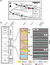 Figure 1.
(A) Location map showing the key structural features of the Alaska North Slope (ANS) and the position of Milne Point. (B) Summary of the ages of the stratigraphic sequences and the formation lithologies that were seismically imaged. The Shublik Formation shale, Kingak Shale, and Pebble shale are highlighted as important source rock formations for the Prudhoe Bay, Milne Point, and Kuparuk River oil fields. The KUP and SAG horizons are indicated as the bottom and top of the Kuparuk River and Sag River reservoir sandstone formations, respectively.
Figure 1.
(A) Location map showing the key structural features of the Alaska North Slope (ANS) and the position of Milne Point. (B) Summary of the ages of the stratigraphic sequences and the formation lithologies that were seismically imaged. The Shublik Formation shale, Kingak Shale, and Pebble shale are highlighted as important source rock formations for the Prudhoe Bay, Milne Point, and Kuparuk River oil fields. The KUP and SAG horizons are indicated as the bottom and top of the Kuparuk River and Sag River reservoir sandstone formations, respectively.
The principal structural features of the region (Figure 1A) are the Barrow Arch to the north, and the Colville Basin and Brooks Range to the south (Carman and Hardwick, 1983; Bird, 1999; Boswell et al., 2011). The Barrow Arch is an east–west–trending rift shoulder and the Brooks Range is a fold and thrust mountain belt related to continent–continent collision (Bird, 1999). Together, these structural highs provided source material that filled the Colville (foreland) Basin, which has an east–west axial trend (Figure 1A) (Carmen and Hardwick, 1983; Bird, 1999).
The sedimentary rocks of the Alaska North Slope consist of south-dipping passive continental margin deposits of late Paleozoic and Mesozoic age, overlain by north-dipping foreland basin deposits in the Mesozoic and Cenozoic (Collett, 1993; Bird, 1999). These deposits have been divided into three main tectono-stratigraphic sequences (Figure 1B) that are described in detail by Bird (1999). The earlier passive-margin deposits are termed the Ellesmerian sequence. These consist of clastic and carbonate strata of middle Devonian to Triassic age, that onlap onto a stable south-facing continental margin (Collett, 1993; Bird, 1999). The Ellesmerian was followed by the Beaufortian sequence that was deposited during a period of continental rifting in the Jurassic and Early Cretaceous (Bird, 1999). The rifting is characterized by south-dipping normal faulting in the Jurassic followed by north-dipping normal faulting in the Early Cretaceous (Hubbard et al., 1987). This rift formed the paleo-high of the Barrow Arch. Then during the Cretaceous and Cenozoic, continent–continent collision caused uplift to the south, that is, the Brooks Range, and subsidence to the north producing the Colville Basin and the foreland basin deposits of the Brookian sequence (Carmen and Hardwick, 1983; Collett 1993; Bird, 1999). The Brookian sequence is also extensively faulted in the Milne Point region by north-northeast-striking normal faults (Boswell et al., 2011; Lorenson et al., 2011). The Jurassic–Cretaceous rift faults and later Brookian faults are likely to have initiated at different burial depths.
The Milne Point Field (Figure 1A) produces from three separate reservoirs: the Schrader Bluff, Kuparuk, and Sag River Formations. The Schrader Bluff is a shallow, unconsolidated viscous oil reservoir. The Sag River is a deeper, Upper Triassic sandstone reservoir with light oil occurring within the Ellesmerian sequence. It is also a reservoir elsewhere in the Prudhoe Bay area and contains gas in the Kavik field southeast of Prudhoe Bay (Bird, 1999). The Kuparuk Formation forms the main reservoir (Figure 1B). This is a Lower Cretaceous, shallow-marine sandstone that hosts several oil reservoirs in northern Alaska, including Milne Point and the neighboring Kuparuk River field (Bird, 1999). Both these accumulations occur in combination structural stratigraphic traps. According to Dzou (2010), the Kuparuk River reservoir was charged from deeper, Shublik Shale source rocks with some gas contribution from Kekiktuk coals. Published resources for Milne Point’s light (American Petroleum Institute [API] 22) oil Kuparuk reservoir are approximately 920 MM (million) stock tank barrels original oil-in-place (Ning and McGuire, 2004). Water-flood assisted production began in 1985.
The ![]() fault
fault![]() network studied in this paper affects the Triassic to Lower Cretaceous rocks (Figures 1B, 2). We concentrate on analyzing the network at two stratigraphic horizons within the 3-D seismic data: the younger horizon that follows the bottom of the Kuparuk Formation (KUP horizon; Figure 1B) and an older horizon that follows the top of the Sag River Formation (SAG horizon; Figure 1B). The orthogonal
network studied in this paper affects the Triassic to Lower Cretaceous rocks (Figures 1B, 2). We concentrate on analyzing the network at two stratigraphic horizons within the 3-D seismic data: the younger horizon that follows the bottom of the Kuparuk Formation (KUP horizon; Figure 1B) and an older horizon that follows the top of the Sag River Formation (SAG horizon; Figure 1B). The orthogonal ![]() fault
fault![]() network cuts both of these reservoir horizons, frequently with displacements exceeding reservoir interval thicknesses. This leads to a range of variable oil–water contacts and closely spaced compartmentalization. Understanding the controls on fluid flow of such a
network cuts both of these reservoir horizons, frequently with displacements exceeding reservoir interval thicknesses. This leads to a range of variable oil–water contacts and closely spaced compartmentalization. Understanding the controls on fluid flow of such a ![]() fault
fault![]() network clearly impacts efficient reserve recovery and well planning.
network clearly impacts efficient reserve recovery and well planning.
 Figure 2.
Seismic reflection images of (A) a northwest–southeast trending crossline and (B) a northeast–southwest trending in line. Red represents the west-northwest–trending
Figure 2.
Seismic reflection images of (A) a northwest–southeast trending crossline and (B) a northeast–southwest trending in line. Red represents the west-northwest–trending ![]() fault
fault![]() set that was picked on the in lines and blue represents the north-northeast–trending
set that was picked on the in lines and blue represents the north-northeast–trending ![]() fault
fault![]() set that was picked on the crosslines. Dashed lines are the faults that were not picked on the in line or crossline but have been projected onto the seismic section. (C) Location map showing the orientation of the in lines and crosslines.
set that was picked on the crosslines. Dashed lines are the faults that were not picked on the in line or crossline but have been projected onto the seismic section. (C) Location map showing the orientation of the in lines and crosslines.
METHODS
Data Acquisition and Interpretation
The 3-D seismic reflection data was acquired using Vibroseis in 2007. The data are of high quality, cover an onshore area at Milne Point of  (
( ) (Figure 1A), and are 120-fold containing frequencies between 6 and 96 Hz. The 3-D migrated seismic volume comprises 1238 inlines bearing N045°E and 897 crosslines bearing N135°E, each with a spacing of 16.8 m (55 ft) (Figure 2). Interval velocities of 3050 m/s (10,007 ft/s) and 4100 m/s (13,451 ft/s) were calculated for the KUP horizon and the SAG horizon, respectively, using true vertical depth subsea (TVDSS) and two-way time (TWT) values taken from geophysical wireline-log well data.
The ![]() fault
fault![]() network was interpreted for a sequence of sedimentary rocks, ∼650 m (2133 ft) thick at a depth greater than 2000 m (6562 ft) (Figure 2). Faults were identified and picked on every tenth inline section (N045°E) and crossline section (N135°E) from offsets of key seismic reflectors. In general, the seismic data imaged faults with >10 m (>32.8 ft) displacement. Using TrapTester, a seismic interpretation and seismic modeling software developed by Badley Geoscience Limited, an interconnected 3-D
network was interpreted for a sequence of sedimentary rocks, ∼650 m (2133 ft) thick at a depth greater than 2000 m (6562 ft) (Figure 2). Faults were identified and picked on every tenth inline section (N045°E) and crossline section (N135°E) from offsets of key seismic reflectors. In general, the seismic data imaged faults with >10 m (>32.8 ft) displacement. Using TrapTester, a seismic interpretation and seismic modeling software developed by Badley Geoscience Limited, an interconnected 3-D ![]() fault
fault![]() model was produced. This involved identifying
model was produced. This involved identifying ![]() fault
fault![]() intersections from displaced raw horizon data for multiple horizons that were then validated using coherency time slices. Branch lines were then created to connect the intersecting
intersections from displaced raw horizon data for multiple horizons that were then validated using coherency time slices. Branch lines were then created to connect the intersecting ![]() fault
fault![]() planes.
planes.
Hanging wall and footwall cutoffs of the KUP and SAG horizons were projected from raw horizon data onto the modeled ![]() fault
fault![]() surfaces. To correct for local effects, such as
surfaces. To correct for local effects, such as ![]() fault
fault![]() drag around
drag around ![]() fault
fault![]() surfaces, the raw horizon data that were within 75 m (246 ft) of each
surfaces, the raw horizon data that were within 75 m (246 ft) of each ![]() fault
fault![]() were trimmed and a 100 m (328 ft) wide patch of horizon data was used to calculate and project each horizon surface onto the
were trimmed and a 100 m (328 ft) wide patch of horizon data was used to calculate and project each horizon surface onto the ![]() fault
fault![]() surface. The interval velocities and the TWT of each hanging wall and footwall cutoff were then used to measure numerous
surface. The interval velocities and the TWT of each hanging wall and footwall cutoff were then used to measure numerous ![]() fault
fault![]() -attribute data (such as displacement, throw, heave, dip, azimuth, and strike) at 100 m (328 ft) intervals along the plan view length of each interpreted
-attribute data (such as displacement, throw, heave, dip, azimuth, and strike) at 100 m (328 ft) intervals along the plan view length of each interpreted ![]() fault
fault![]() surface.
surface.
Network Analysis
The ![]() fault
fault![]() attribute data were extracted from TrapTester software, with associated
attribute data were extracted from TrapTester software, with associated  and
and  coordinates. The data were imported into ArcGIS as point data and used to digitize
 ![]() fault
fault![]() traces to produce
traces to produce ![]() fault
fault![]() maps for both the KUP and SAG horizons. Each
maps for both the KUP and SAG horizons. Each ![]() fault
fault![]() trace was split into shorter segments (∼100 m [328 ft] in length) at each
trace was split into shorter segments (∼100 m [328 ft] in length) at each ![]() fault
fault![]() attribute data point. Average throws and segment azimuths were calculated allowing the network to be displayed by
attribute data point. Average throws and segment azimuths were calculated allowing the network to be displayed by ![]() fault
fault![]() trend and
trend and ![]() fault
fault![]() throw. The
throw. The ![]() fault
fault![]() maps combined with length-weighted rose diagrams,
maps combined with length-weighted rose diagrams, ![]() fault
fault![]() length vs.
length vs. ![]() fault
fault![]() throw plots and
throw plots and ![]() fault
fault![]() throw profiles were used to investigate the geometry, kinematics, and interactions within the
throw profiles were used to investigate the geometry, kinematics, and interactions within the ![]() fault
fault![]() network.
network.
In addition, 3-D strain was calculated to assess the partitioning of deformation within the ![]() fault
fault![]() network. This uses the
network. This uses the ![]() fault
fault![]() orientation and dip separation to construct the Lagrangian strain tensor, as described by Peacock and Sanderson (1993) and Nixon et al. (2011). This involves calculating the eigenvalues and eigenvectors of the Lagrangian strain tensor (
orientation and dip separation to construct the Lagrangian strain tensor, as described by Peacock and Sanderson (1993) and Nixon et al. (2011). This involves calculating the eigenvalues and eigenvectors of the Lagrangian strain tensor ( ) when sampling faults from a
 ![]() plane
plane![]() :
: 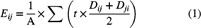
in which  is the sample area,
  is the
 ![]() fault
fault![]() trace-length, and
trace-length, and  is the displacement tensor, and
  is the transpose. Although interactions within normal-
![]() fault
fault![]() networks often produce complex 3-D strains, which are supported by simple geometric models (e.g., Ferrill and Morris, 2001) as well as numerical models (e.g., Imber et al., 2004; Goteti et al., 2013), no slip direction data exists for the normal faults observed in the 3-D seismic reflection data at Milne Point. Therefore, as these are normal faults, and we are considering the entirety of the
networks often produce complex 3-D strains, which are supported by simple geometric models (e.g., Ferrill and Morris, 2001) as well as numerical models (e.g., Imber et al., 2004; Goteti et al., 2013), no slip direction data exists for the normal faults observed in the 3-D seismic reflection data at Milne Point. Therefore, as these are normal faults, and we are considering the entirety of the ![]() fault
fault![]() network, we assume dip-slip displacement and apply a weighting factor (
network, we assume dip-slip displacement and apply a weighting factor ( ) defined by Peacock and Sanderson (1993) to the displacement tensor, which corrects for the orientation bias between the sample
 ![]() plane
plane![]() and the dip angle (θ) of the faults, hence:
and the dip angle (θ) of the faults, hence: 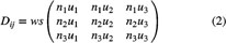
in which  is the displacement and unit vectors
  and
and  are normal to the
 ![]() fault
fault![]()
![]() plane
plane![]() and parallel to the slip direction, respectively. As we assume dip-slip movement on these faults, in which faults have a dip angle (θ) and a dip direction (Φ), then:
and parallel to the slip direction, respectively. As we assume dip-slip movement on these faults, in which faults have a dip angle (θ) and a dip direction (Φ), then: 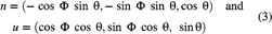
FAULT NETWORK CHARACTERISTICS
General Structural Trends and Relationships
The study area has an underlying structural grain trending northwest-southeast which forms broad-scale graben and horst structures on both horizons (Figure 3A). These are particularly well defined in the deeper SAG horizon and coincide with an overall deepening to the east-northeast of ∼490 m (1608 ft) in the KUP horizon and ∼615 m (2018 ft) in the SAG horizon. The ![]() fault
fault![]() network overprints this structural grain and has two sets of normal faults, a north-northeast-trending set and a west-northwest–trending set (Figures 3B, 4).
network overprints this structural grain and has two sets of normal faults, a north-northeast-trending set and a west-northwest–trending set (Figures 3B, 4).
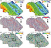 Figure 3.
![]() Fault
Fault![]() maps of the KUP horizon on the left and the SAG horizon on the right: (A) Surface horizon maps showing the topography of the horizons; (B)
maps of the KUP horizon on the left and the SAG horizon on the right: (A) Surface horizon maps showing the topography of the horizons; (B) ![]() fault
fault![]() map color-coded by azimuth with red generally representing west-northwest–faults and blue generally representing north-northeast-faults; (C)
map color-coded by azimuth with red generally representing west-northwest–faults and blue generally representing north-northeast-faults; (C) ![]() fault
fault![]() map color-coded by throw with blue and orange representing low- and high-throw values, respectively. The location of specific
map color-coded by throw with blue and orange representing low- and high-throw values, respectively. The location of specific ![]() fault
fault![]() maps and 3-D diagrams used in later figures are also shown.
maps and 3-D diagrams used in later figures are also shown.
 Figure 4.
Length-weighted rose diagrams and an equal-angle stereographic projection of poles to
Figure 4.
Length-weighted rose diagrams and an equal-angle stereographic projection of poles to ![]() fault
fault![]() segments for each
segments for each ![]() fault
fault![]() set in the KUP horizon (top) and SAG horizon (bottom).
set in the KUP horizon (top) and SAG horizon (bottom).
The north-northeast–trending faults are regularly spaced (1–2 km [0.6–1.2 mi]) and most down throw to the southeast (Figures 2A, 4) with constant dips of ∼50–60°. They displace both the KUP and SAG horizons by similar amounts (Figures 2A, 5A); therefore, these are post-depositional, as indicated by the constant thickness of stratigraphy across each ![]() fault
fault![]() (Figure 5A).
(Figure 5A).
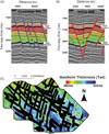 Figure 5.
Interpreted seismic sections showing the stratigraphic thickness in relation to (A) the north-northeast–trending faults and (B) the west-northwest–trending faults. (C) An isochore map showing the variation in stratigraphic thickness (two-way time [TWT]) between the KUP and SAG horizons. The black patches cover the areas that have been tectonically thinned by throughgoing faults.
Figure 5.
Interpreted seismic sections showing the stratigraphic thickness in relation to (A) the north-northeast–trending faults and (B) the west-northwest–trending faults. (C) An isochore map showing the variation in stratigraphic thickness (two-way time [TWT]) between the KUP and SAG horizons. The black patches cover the areas that have been tectonically thinned by throughgoing faults.
The majority of the faults in the west-northwest–trending ![]() fault
fault![]() set dip to the southwest (Figures 2B, 4). Unlike the north-northeast–trending faults these are not regularly spaced and many of the larger faults become steeper at depth with dips increasing from ∼40–50° to ∼70–80° (Figures 2B, 5B). Furthermore, the west-northwest–trending faults often displace the SAG horizon more than the KUP horizon (Figures 2B, 5B) and, hence, have a component of syndepositional movement associated with them (i.e., thickening of stratigraphic sequence 4; Figure 5B). Overall the stratigraphic thickness between the KUP and SAG horizons increases from a minimum of ∼325 ms (TWT) in the north to a maximum of ∼425 ms (TWT) in the south of the study area and is not related to syndepositional sedimentation associated with either
set dip to the southwest (Figures 2B, 4). Unlike the north-northeast–trending faults these are not regularly spaced and many of the larger faults become steeper at depth with dips increasing from ∼40–50° to ∼70–80° (Figures 2B, 5B). Furthermore, the west-northwest–trending faults often displace the SAG horizon more than the KUP horizon (Figures 2B, 5B) and, hence, have a component of syndepositional movement associated with them (i.e., thickening of stratigraphic sequence 4; Figure 5B). Overall the stratigraphic thickness between the KUP and SAG horizons increases from a minimum of ∼325 ms (TWT) in the north to a maximum of ∼425 ms (TWT) in the south of the study area and is not related to syndepositional sedimentation associated with either ![]() fault
fault![]() trend (Figure 5C).
trend (Figure 5C).
Because of the downward increase in throw and resultant hanging-wall thickening (Figure 5B), the west-northwest–trending faults are suggested to be associated with rifting during the deposition of the Beaufortian sequence (Jurassic to Lower Cretaceous). The majority of these faults dip south, consistent with the polarity of Jurassic rifting observed elsewhere on the Alaska North Slope (Hubbard et al., 1987; Bird, 1999). Abutting and cross-cutting relationships indicate that the north-northeast–trending faults postdate many of the west-northwest–trending faults (Figure 3), which is supported by the north-northeast–trending faults consistent with those that cut the Brookian sequence in the Cenozoic (Boswell et al., 2011), which have been shown to cut the top of the Kuparuk Formation (Masterson et al., 2001).
Later local reactivation of the west-northwest–trending faults, related to changes in regional and/or local stress orientations, is supported by the fact that some of the north-northeast–trending faults are abutted by some small west-northwest–trending faults (Figure 3). This is also consistent with the presence of small faults and ![]() fault
fault![]() splays that trend approximately northwest–southeast in the Eocene Sagavanirktok Formation (Boswell et al., 2011; Lorenson et al., 2011), which are thought to be genetically linked to the underlying faults (Collett et al., 2011). Furthermore, the present-day stress regime of the area favors the reactivation of the west-northwest–trending faults (Zoback, 1992; Heidbach et al., 2010).
splays that trend approximately northwest–southeast in the Eocene Sagavanirktok Formation (Boswell et al., 2011; Lorenson et al., 2011), which are thought to be genetically linked to the underlying faults (Collett et al., 2011). Furthermore, the present-day stress regime of the area favors the reactivation of the west-northwest–trending faults (Zoback, 1992; Heidbach et al., 2010).
Organization of Faulting and Throw Distribution
Many of the large west-northwest–trending faults are aligned with or influenced by the underlying northwest–southeast structural grain. This is more obvious in the deeper SAG horizon where large faults from the west-northwest–trending ![]() fault
fault![]() set bound many of the graben structures (Figure 3A). In addition, en echelon arrays of smaller west-northwest–trending faults form above the underlying northwest-southeast structures and often splay from/rotate into the larger graben-bounding faults (Figure 3B). This influence becomes more emphatic with depth where the trend of the west-northwest–trending faults is oriented ∼10° farther clockwise in the deeper SAG horizon, which can be seen clearly in the length-weighted rose diagrams (Figure 4C, F).
set bound many of the graben structures (Figure 3A). In addition, en echelon arrays of smaller west-northwest–trending faults form above the underlying northwest-southeast structures and often splay from/rotate into the larger graben-bounding faults (Figure 3B). This influence becomes more emphatic with depth where the trend of the west-northwest–trending faults is oriented ∼10° farther clockwise in the deeper SAG horizon, which can be seen clearly in the length-weighted rose diagrams (Figure 4C, F).
The west-northwest–trending faults also become more pervasive with depth increasing in density from  (
( ) in the KUP to
  (
( ) in the SAG horizon (Table 1). In contrast, the north-northeast–trending faults have similar
 ![]() fault
fault![]() density values for each horizon (i.e.,
density values for each horizon (i.e.,  [
[ ] at the KUP horizon and
  [
[ ] at the SAG horizon; Table 1). As a result, the KUP horizon has approximately equal proportions of north-northeast–trending and west-northwest–trending faults, whereas the SAG horizon has an increased proportion of west-northwest–trending faults (∼64%; Table 1).
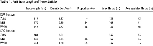
The largest faults in the network trend west-northwest with maximum throws of up to 138 m (453 ft) in the KUP horizon and 332 m (1089 ft) in the SAG horizon (Table 1; Figure 3C). In general, the maximum throw of faults increases from the shallower KUP horizon to the deeper SAG horizon (Figure 6A). This increase is seen mainly in the west-northwest–trending faults (Figure 6C) as indicated by the average maximum throw values for each ![]() fault
fault![]() set (Table 1).
set (Table 1).
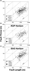 Figure 6.
Logarithmic plots of
Figure 6.
Logarithmic plots of ![]() fault
fault![]() length versus maximum throw for (A) all faults, (B) the KUP horizon, and (C) the SAG horizon. Note the significantly greater throws for some west-northwest–trending faults in the SAG horizon.
length versus maximum throw for (A) all faults, (B) the KUP horizon, and (C) the SAG horizon. Note the significantly greater throws for some west-northwest–trending faults in the SAG horizon.
In summary, the north-northeast–trending faults are evenly distributed both in space and with depth showing similar orientations, ![]() fault
fault![]() densities, and throws for each horizon. In contrast, the west-northwest–trending faults increase in density, size, and dip with depth. They also become more parallel to the underlying structural grain, suggesting influence of deeper pre-existing structures.
densities, and throws for each horizon. In contrast, the west-northwest–trending faults increase in density, size, and dip with depth. They also become more parallel to the underlying structural grain, suggesting influence of deeper pre-existing structures.
Strain Analysis
Each ![]() fault
fault![]() trend has a narrow range of strike orientations and shows negligible amounts of extension for the intermediate strain component (Figure 7A, B; Table 2). The north-northeast–trending faults accommodate similar amounts of extension in each horizon, whereas the maximum extension that is accommodated by the west-northwest–trending faults increases in the SAG horizon (Table 2). Hence, in the SAG horizon the majority of the strain (69%) is accommodated by the west-northwest–trending faults.
trend has a narrow range of strike orientations and shows negligible amounts of extension for the intermediate strain component (Figure 7A, B; Table 2). The north-northeast–trending faults accommodate similar amounts of extension in each horizon, whereas the maximum extension that is accommodated by the west-northwest–trending faults increases in the SAG horizon (Table 2). Hence, in the SAG horizon the majority of the strain (69%) is accommodated by the west-northwest–trending faults.
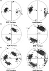 Figure 7.
Equal-angle stereographic projection of poles to
Figure 7.
Equal-angle stereographic projection of poles to ![]() fault
fault![]() segments showing the principal strain orientations for (A) the north-northeast–trending faults, (B) the west-northwest–trending faults, and (C) all faults.
segments showing the principal strain orientations for (A) the north-northeast–trending faults, (B) the west-northwest–trending faults, and (C) all faults.
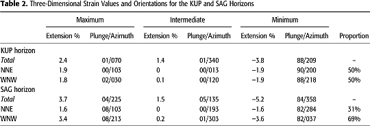
Like the strain accommodated by the individual ![]() fault
fault![]() trends, the overall composite strain of the
trends, the overall composite strain of the ![]() fault
fault![]() network indicates subhorizontal extension and subvertical shortening at each horizon (Figure 7; Table 2). The maximum extension accommodated by the
network indicates subhorizontal extension and subvertical shortening at each horizon (Figure 7; Table 2). The maximum extension accommodated by the ![]() fault
fault![]() network increases from 2.4% oriented at N70°E for the KUP horizon to 3.7% oriented at N225°E for the SAG horizon (Table 2), which is accommodated entirely by the west-northwest–trending faults. As the strain accommodated by the
network increases from 2.4% oriented at N70°E for the KUP horizon to 3.7% oriented at N225°E for the SAG horizon (Table 2), which is accommodated entirely by the west-northwest–trending faults. As the strain accommodated by the ![]() fault
fault![]() network is a superposition of the two strains accommodated by each
network is a superposition of the two strains accommodated by each ![]() fault
fault![]() trend, which are orthogonal to one another, an intermediate strain component also exists with an extension of ∼1.5% oriented at N340°E and N135°E for the KUP and SAG horizons, respectively. In the KUP horizon, the total strain is accommodated equally between the two
trend, which are orthogonal to one another, an intermediate strain component also exists with an extension of ∼1.5% oriented at N340°E and N135°E for the KUP and SAG horizons, respectively. In the KUP horizon, the total strain is accommodated equally between the two ![]() fault
fault![]() trends, as indicated by the minimum extension percentages (Table 2), resulting in the maximum extension direction of the network approximately bisecting the angle of intersection between the two
trends, as indicated by the minimum extension percentages (Table 2), resulting in the maximum extension direction of the network approximately bisecting the angle of intersection between the two ![]() fault
fault![]() trends (east-northeast–west-southwest; Figure 7C). However, in the SAG horizon the network’s maximum extension direction is rotated 25° counterclockwise to approximately northeast–southwest (Table 2; Figure 7C), as more of the total extension is produced by the west-northwest–trending faults.
trends (east-northeast–west-southwest; Figure 7C). However, in the SAG horizon the network’s maximum extension direction is rotated 25° counterclockwise to approximately northeast–southwest (Table 2; Figure 7C), as more of the total extension is produced by the west-northwest–trending faults.
In general, the strain analysis shows an increase in strain with depth because of more strain being localized onto the west-northwest–trending faults in the deeper SAG horizon. The contrast between the behavior of the two ![]() fault
fault![]() sets indicates that they are independent
sets indicates that they are independent ![]() fault
fault![]() sets. In addition, localization of strain onto the west-northwest–trending faults further suggests that these faults are being influenced by the pre-existing structures that form the northwest–southeast underlying structural grain.
sets. In addition, localization of strain onto the west-northwest–trending faults further suggests that these faults are being influenced by the pre-existing structures that form the northwest–southeast underlying structural grain.
INDIVIDUAL FAULTS AND SPLAYS
Isolated Faults
Very few isolated faults exist within the ![]() fault
fault![]() network at Milne Point, and these are mostly small faults with lengths ranging from approximately 400 to 1700 m (1312 to 5577 ft) accumulating maximum throws of less than 50 m (164 ft). Throw profiles of the isolated faults can be divided into three main groups: Unrestricted, single-tip restricted, and double-tip restricted (Figure 8) (compare Nicol et al., 1996; Manighetti et al., 2001; Soliva and Benedicto, 2005).
network at Milne Point, and these are mostly small faults with lengths ranging from approximately 400 to 1700 m (1312 to 5577 ft) accumulating maximum throws of less than 50 m (164 ft). Throw profiles of the isolated faults can be divided into three main groups: Unrestricted, single-tip restricted, and double-tip restricted (Figure 8) (compare Nicol et al., 1996; Manighetti et al., 2001; Soliva and Benedicto, 2005).
 Figure 8.
Normalized
Figure 8.
Normalized ![]() fault
fault![]() profiles for isolated faults from both the KUP and SAG horizons with length/maximum length (
profiles for isolated faults from both the KUP and SAG horizons with length/maximum length ( ) along the x axis versus throw/maximum throw (
 ) on the y axis. (A) Isolated faults with unrestricted tips; (B) isolated faults with a single tip restricted; (C) isolated faults with both tips restricted. The graphs on the right side are cartoon representations of each
 ![]() profile
profile![]() .
.
The examples in Figure 8A are symmetrical profiles with the maximum throw located near the center of the ![]() fault
fault![]() . These either match that of an ideal elastic
. These either match that of an ideal elastic ![]() profile
profile![]() , as modeled for fractures in a homogenous material by Pollard and Segall (1987), or a symmetrical cone-shaped
, as modeled for fractures in a homogenous material by Pollard and Segall (1987), or a symmetrical cone-shaped ![]() profile
profile![]() , as described by Muraoka and Kamata (1983) for faults that form in incompetent layers. Such profiles have been shown to be characteristic of faults with unrestricted tips (compare Nicol et al., 1996, 2010; Manighetti et al., 2001) and are the smallest isolated faults within the network as indicated by their average maximum throw and average length (Figure 8A).
, as described by Muraoka and Kamata (1983) for faults that form in incompetent layers. Such profiles have been shown to be characteristic of faults with unrestricted tips (compare Nicol et al., 1996, 2010; Manighetti et al., 2001) and are the smallest isolated faults within the network as indicated by their average maximum throw and average length (Figure 8A).
Other profiles are asymmetrical with the maximum throw located closer to one of the ![]() fault
fault![]() tips producing a tip with a steep throw-length gradient (Figure 8B). These profiles match the single-tip and half-restricted
tips producing a tip with a steep throw-length gradient (Figure 8B). These profiles match the single-tip and half-restricted ![]() fault
fault![]() -displacement profiles described in Manighetti et al. (2001). These are not caused by
-displacement profiles described in Manighetti et al. (2001). These are not caused by ![]() fault
fault![]() abutments but either by lithological barriers (such as changes in competency) or by soft linkage with nearby faults that restrict the propagation rate of a
abutments but either by lithological barriers (such as changes in competency) or by soft linkage with nearby faults that restrict the propagation rate of a ![]() fault
fault![]() tip indicating kinematic interaction between faults (e.g., relay ramps) (Peacock and Sanderson, 1996; Schlagenhauf et al., 2008; Nicol et al., 2010).
tip indicating kinematic interaction between faults (e.g., relay ramps) (Peacock and Sanderson, 1996; Schlagenhauf et al., 2008; Nicol et al., 2010).
The majority of isolated faults at Milne Point produce a symmetrical ![]() profile
profile![]() with a flat top and steep gradients at each
with a flat top and steep gradients at each ![]() fault
fault![]() tip (Figure 8C). Such a shape in
tip (Figure 8C). Such a shape in ![]() fault
fault![]() -displacement profiles has been described in numerous studies (Muraoka and Kamata, 1983; Peacock and Sanderson, 1991; Manighetti et al., 2001; Nicol et al., 2010). Muraoka and Kamata (1983) describe these as a mesa-shaped
-displacement profiles has been described in numerous studies (Muraoka and Kamata, 1983; Peacock and Sanderson, 1991; Manighetti et al., 2001; Nicol et al., 2010). Muraoka and Kamata (1983) describe these as a mesa-shaped ![]() profile
profile![]() for faults that form with tips that terminate in strain-absorbing incompetent stratigraphic layering. Hence, these are double-tip restricted-
for faults that form with tips that terminate in strain-absorbing incompetent stratigraphic layering. Hence, these are double-tip restricted-![]() fault
fault![]() profiles and have the largest average maximum throw and average-length values of the isolated faults.
profiles and have the largest average maximum throw and average-length values of the isolated faults.
In summary, the isolated faults within the network have isolated tips and produce common throw-length profiles the shape of which depends on the restriction of the ![]() fault
fault![]() tips (Muraoka and Kamata, 1983; Pollard and Segall, 1987; Nicol et al., 1996, 2010; Manighetti et al., 2001; Schlagenhauf et al., 2008). In general,
tips (Muraoka and Kamata, 1983; Pollard and Segall, 1987; Nicol et al., 1996, 2010; Manighetti et al., 2001; Schlagenhauf et al., 2008). In general, ![]() fault
fault![]() -tip restriction is characterized by a high throw gradient at the restricted tip.
-tip restriction is characterized by a high throw gradient at the restricted tip.
Individual Faults
Although the isolated faults have short lengths (less than 2000 m [6562 ft]), many of the faults within the network have longer ![]() fault
fault![]() lengths (up to 9000 m [29,528 ft]) and accumulate much larger throws (Figures 3, 6). These longer faults are often segmented by cross-cutting faults or have numerous faults that abut them (Figure 3). Even though these long faults are segmented by many intersecting faults, the displacement variations along their
lengths (up to 9000 m [29,528 ft]) and accumulate much larger throws (Figures 3, 6). These longer faults are often segmented by cross-cutting faults or have numerous faults that abut them (Figure 3). Even though these long faults are segmented by many intersecting faults, the displacement variations along their ![]() fault
fault![]() planes are consistent with each other (Figure 9A). Hence, their throw profiles are often symmetrical with maximum throws near the center of the
planes are consistent with each other (Figure 9A). Hence, their throw profiles are often symmetrical with maximum throws near the center of the ![]() fault
fault![]()
![]() plane
plane![]() and minimum throws at their tips (Figure 9), which is similar to throw profiles of isolated faults.
and minimum throws at their tips (Figure 9), which is similar to throw profiles of isolated faults.
As each segment has a displacement ![]() profile
profile![]() that is consistent with its adjacent segment, these can be considered as coherent structures and not isolated
that is consistent with its adjacent segment, these can be considered as coherent structures and not isolated ![]() fault
fault![]() segments that have aligned and linked (compare Walsh et al., 2003). Therefore, despite interactions with other
segments that have aligned and linked (compare Walsh et al., 2003). Therefore, despite interactions with other ![]() fault
fault![]() sets the larger and longer faults still act as individual isolated faults. This can be identified for both
sets the larger and longer faults still act as individual isolated faults. This can be identified for both ![]() fault
fault![]() sets and indicates that the faults in both sets originally developed as individual faults rather than simultaneously.
sets and indicates that the faults in both sets originally developed as individual faults rather than simultaneously.
 Figure 9.
![]() Fault
Fault![]() -throw profiles of long individual faults (>2000 m [>6562 ft] length) which have numerous intersecting and abutting faults. (A) A 3-D diagram of an individual west-northwest–trending
-throw profiles of long individual faults (>2000 m [>6562 ft] length) which have numerous intersecting and abutting faults. (A) A 3-D diagram of an individual west-northwest–trending ![]() fault
fault![]()
![]() plane
plane![]() (
(![]() fault
fault![]() 11-KUP) in the KUP horizon with throw contoured onto the
11-KUP) in the KUP horizon with throw contoured onto the ![]() fault
fault![]()
![]() plane
plane![]() ; (B) a throw
; (B) a throw ![]() profile
profile![]() along the length of
along the length of ![]() fault
fault![]() 11-KUP (see Figure 3C for location within the
11-KUP (see Figure 3C for location within the ![]() fault
fault![]() network); and (C) normalized throw profiles of numerous long individual faults within the network. Examples are taken from both the KUP and SAG horizons. Note the similarity to isolated-
network); and (C) normalized throw profiles of numerous long individual faults within the network. Examples are taken from both the KUP and SAG horizons. Note the similarity to isolated-![]() fault
fault![]() throw-length profiles.
throw-length profiles.
Splays
![]() Fault
Fault![]() splays often occur near the tips of faults and involve a smaller
splays often occur near the tips of faults and involve a smaller ![]() fault
fault![]() that splays away from a larger
that splays away from a larger ![]() fault
fault![]() . The smaller splay
. The smaller splay ![]() fault
fault![]() has a
has a ![]() fault
fault![]()
![]() plane
plane![]() that is obliquely oriented to the larger main
that is obliquely oriented to the larger main ![]() fault
fault![]()
![]() plane
plane![]() and has a displacement maximum along the line of intersection (Figure 10A). The displacement distribution on the
and has a displacement maximum along the line of intersection (Figure 10A). The displacement distribution on the ![]() fault
fault![]()
![]() plane
plane![]() of the main
of the main ![]() fault
fault![]() shows an abrupt drop in displacement at the line of intersection with the splay
shows an abrupt drop in displacement at the line of intersection with the splay ![]() fault
fault![]() (Figure 10A).
(Figure 10A).
 Figure 10.
(A) A 3-D diagram showing the distribution of throw on the
Figure 10.
(A) A 3-D diagram showing the distribution of throw on the ![]() fault
fault![]() planes of a splay
planes of a splay ![]() fault
fault![]() (
(![]() fault
fault![]() 100-KUP) and its associated main
100-KUP) and its associated main ![]() fault
fault![]() (
(![]() fault
fault![]() 99-KUP). Panels (B) and (C) are
99-KUP). Panels (B) and (C) are ![]() fault
fault![]() profiles of a main
profiles of a main ![]() fault
fault![]() and a splay
and a splay ![]() fault
fault![]() showing their variations in throw along distance X, which increases to the east. To the right of each graph are plan-view
showing their variations in throw along distance X, which increases to the east. To the right of each graph are plan-view ![]() fault
fault![]() maps of the interacting faults. See Figure 3C for the locations of these faults within the
maps of the interacting faults. See Figure 3C for the locations of these faults within the ![]() fault
fault![]() network.
network.
![]() Fault
Fault![]() -throw profiles indicate that the decrease in displacement is accommodated by the splay
-throw profiles indicate that the decrease in displacement is accommodated by the splay ![]() fault
fault![]() . For example, Figure 10B and C show the throw profiles of two main faults (99-KUP and 57-SAG) that have corresponding splays (faults 100-KUP and 177-SAG) at intersection points A and B, respectively. Both of the main faults show a step-like decrease in throw at the intersection with the splay faults in the direction of the acute angle of intersection. This step down in throw approximately matches the throw of the respective splay faults near the point of intersection (Figure 10). After the point of intersection both the main
. For example, Figure 10B and C show the throw profiles of two main faults (99-KUP and 57-SAG) that have corresponding splays (faults 100-KUP and 177-SAG) at intersection points A and B, respectively. Both of the main faults show a step-like decrease in throw at the intersection with the splay faults in the direction of the acute angle of intersection. This step down in throw approximately matches the throw of the respective splay faults near the point of intersection (Figure 10). After the point of intersection both the main ![]() fault
fault![]() and splay
and splay ![]() fault
fault![]() steadily decrease in throw before reaching null values at their isolated
steadily decrease in throw before reaching null values at their isolated ![]() fault
fault![]() tips. This is consistent with results of Maerten et al. (1999), who observe and model similar throw profiles for splays along normal faults in both plan view and cross section.
tips. This is consistent with results of Maerten et al. (1999), who observe and model similar throw profiles for splays along normal faults in both plan view and cross section.
Overall, the splay faults are characterized by a throw maximum at the point of intersection, with the throw gradually decreasing toward their tips, and they accommodate decreases in throw along a larger main ![]() fault
fault![]() with which they share an intersection line (Figure 10). Nixon et al. (2011) describe
with which they share an intersection line (Figure 10). Nixon et al. (2011) describe ![]() fault
fault![]() splays in strike-slip faults as synthetic interactions that also accommodate a decrease in displacement on a larger main
splays in strike-slip faults as synthetic interactions that also accommodate a decrease in displacement on a larger main ![]() fault
fault![]() . The
. The ![]() fault
fault![]() splays identified in the normal-
splays identified in the normal-![]() fault
fault![]() network at Milne Point accommodate similar decreases in
network at Milne Point accommodate similar decreases in ![]() fault
fault![]() throw (Figure 10) and have the same motion sense (i.e., downthrown on the same side) as their corresponding main faults. Hence, they are called synthetic interactions.
throw (Figure 10) and have the same motion sense (i.e., downthrown on the same side) as their corresponding main faults. Hence, they are called synthetic interactions.
ABUTTING FAULTS AND TRAILING
Abutments
When a ![]() fault
fault![]() network has two or more
network has two or more ![]() fault
fault![]() sets, the tip of one
sets, the tip of one ![]() fault
fault![]() often abuts and terminates against another. This produces a Y- or T-shaped intersection (Figure 11) in which the abutting
often abuts and terminates against another. This produces a Y- or T-shaped intersection (Figure 11) in which the abutting ![]() fault
fault![]() becomes pinned and can only propagate away from its abutted tip. Manighetti et al. (2001) describe these faults as single-tip restricted or half-tip restricted; however, we consider abutting faults to be separate from faults with restricted tips. This is because an abutting tip is actually pinned and cannot propagate any further, whereas a restricted-
becomes pinned and can only propagate away from its abutted tip. Manighetti et al. (2001) describe these faults as single-tip restricted or half-tip restricted; however, we consider abutting faults to be separate from faults with restricted tips. This is because an abutting tip is actually pinned and cannot propagate any further, whereas a restricted-![]() fault
fault![]() tip can still propagate at low propagation rates.
tip can still propagate at low propagation rates.
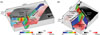 Figure 11.
Three-dimensional diagrams of
Figure 11.
Three-dimensional diagrams of ![]() fault
fault![]() planes that form abutting interactions: (A) an example of an abutting
planes that form abutting interactions: (A) an example of an abutting ![]() fault
fault![]() that shares a footwall block with the main
that shares a footwall block with the main ![]() fault
fault![]() at the SAG horizon; (B) an example of an abutting
at the SAG horizon; (B) an example of an abutting ![]() fault
fault![]() that shares a hanging-wall block with the main
that shares a hanging-wall block with the main ![]() fault
fault![]() at the KUP horizon. Throws are contoured onto each
at the KUP horizon. Throws are contoured onto each ![]() fault
fault![]()
![]() plane
plane![]() showing displacement transfer from the abutting
showing displacement transfer from the abutting ![]() fault
fault![]() to the main
to the main ![]() fault
fault![]() . See Figure 3C for the locations of these faults within the
. See Figure 3C for the locations of these faults within the ![]() fault
fault![]() network.
network.
There are two geometrical relationships that abutting faults form with the earlier abutted ![]() fault
fault![]() (Figure 11). They can either form in the footwall (Figure 11A) or the hanging wall (Figure 11B) of the earlier
(Figure 11). They can either form in the footwall (Figure 11A) or the hanging wall (Figure 11B) of the earlier ![]() fault
fault![]() sharing a footwall or hanging-wall block, respectively. Abutting faults also have the possibility of interacting and transferring displacement onto the earlier
sharing a footwall or hanging-wall block, respectively. Abutting faults also have the possibility of interacting and transferring displacement onto the earlier ![]() fault
fault![]() , thus allowing displacement to build up at the abutting tip (e.g., Maerten, 2000; Maerten et al., 2001). This is accommodated by local reactivation of the earlier
, thus allowing displacement to build up at the abutting tip (e.g., Maerten, 2000; Maerten et al., 2001). This is accommodated by local reactivation of the earlier ![]() fault
fault![]() and can cause local variations in throw adjacent to the intersection line (Figure 11). In general, the earlier
and can cause local variations in throw adjacent to the intersection line (Figure 11). In general, the earlier ![]() fault
fault![]() will locally increase in throw where it shares a
will locally increase in throw where it shares a ![]() fault
fault![]() block with the abutting
block with the abutting ![]() fault
fault![]() (Figure 11).
(Figure 11).
The abutting faults can either be single-tip abutting (Figure 12) or double-tip abutting (Figure 13). Within the ![]() fault
fault![]() network at Milne Point, these are small faults with lengths less than 2000 m (6562 ft). In general, single-tip abutting faults can be divided into two groups, which are shown in Figure 12. Group 1 has minimum throws at its isolated and abutting tips, suggesting that these faults abutted at a late stage of their development. This is supported by the average
network at Milne Point, these are small faults with lengths less than 2000 m (6562 ft). In general, single-tip abutting faults can be divided into two groups, which are shown in Figure 12. Group 1 has minimum throws at its isolated and abutting tips, suggesting that these faults abutted at a late stage of their development. This is supported by the average ![]() fault
fault![]() lengths, which are longer than other
lengths, which are longer than other ![]() profile
profile![]() types for single-tip abutting faults (Figure 12). Therefore,
types for single-tip abutting faults (Figure 12). Therefore, ![]() profile
profile![]() types 1A and 1B are abutting faults that have preserved their isolated
types 1A and 1B are abutting faults that have preserved their isolated ![]() fault
fault![]() throw profiles for unrestricted and single-tip restricted faults, respectively (Figure 12A, B).
throw profiles for unrestricted and single-tip restricted faults, respectively (Figure 12A, B).
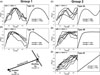 Figure 12.
Normalized
Figure 12.
Normalized ![]() fault
fault![]() profiles of length/maximum length (
profiles of length/maximum length ( ) against throw/maximum throw (
 ) for single-tip abutting faults taken from both the KUP and SAG horizons with no intersections with other faults. Five
 ![]() profile
profile![]() types are identified and divided into two groups. The right graph for each
types are identified and divided into two groups. The right graph for each ![]() profile
profile![]() type is a cartoon representation. See text for discussion.
type is a cartoon representation. See text for discussion.
 Figure 13.
Normalized
Figure 13.
Normalized ![]() fault
fault![]() profiles of length/maximum length (
profiles of length/maximum length ( ) against throw/maximum throw (
 ) for double-tip abutting faults taken from both the KUP and SAG horizons with no intersections with other faults. Four
 ![]() profile
profile![]() types are identified and divided into two groups. The right graph for each
types are identified and divided into two groups. The right graph for each ![]() profile
profile![]() type is a cartoon representation. See text for discussion.
type is a cartoon representation. See text for discussion.
Group 2 has shorter average lengths than Group 1 with maximum throws at the abutting tips. This indicates that the faults have grown in size while being pinned by their abutments, thus interacting with the earlier ![]() fault
fault![]() .
. ![]() Profile
Profile![]() type 2A is thought to represent a
type 2A is thought to represent a ![]() fault
fault![]() at an intermediate stage of development as it still inherits parts of a previous isolated-
at an intermediate stage of development as it still inherits parts of a previous isolated-![]() fault
fault![]()
![]() profile
profile![]() (Figure 12C). However, types 2B and 2C are abutting faults with a restricted tip (flat top; Figure 12D) and unrestricted tip (linear; Figure 12E), respectively, that have grown and propagated since abutting another
(Figure 12C). However, types 2B and 2C are abutting faults with a restricted tip (flat top; Figure 12D) and unrestricted tip (linear; Figure 12E), respectively, that have grown and propagated since abutting another ![]() fault
fault![]() .
.
Double-tip-abutting faults also display two groups of ![]() fault
fault![]() -throw
-throw ![]() profile
profile![]() (Figure 13). Group 1 preserves the throw
(Figure 13). Group 1 preserves the throw ![]() profile
profile![]() of an isolated
of an isolated ![]() fault
fault![]() with both abutting tips recording minimum throws (Figures 13A, B). This suggests that these faults abutted at the late stages of
with both abutting tips recording minimum throws (Figures 13A, B). This suggests that these faults abutted at the late stages of ![]() fault
fault![]() development. Group 2 represents a slightly more developed double-tip-abutting
development. Group 2 represents a slightly more developed double-tip-abutting ![]() fault
fault![]() that has accumulated throws while being pinned at each abutting tip. Hence, these show a maximum throw either at one abutting tip (Figure 13C) or at both
that has accumulated throws while being pinned at each abutting tip. Hence, these show a maximum throw either at one abutting tip (Figure 13C) or at both ![]() fault
fault![]() tips (Figure 13D). The asymmetry of the throw profiles could be caused by the abutting tip with the largest throw value having abutted first.
tips (Figure 13D). The asymmetry of the throw profiles could be caused by the abutting tip with the largest throw value having abutted first.
Overall, the profiles of abutting faults can indicate the relative time of abutment during the faults’ growth and development. Using these numerous throw profiles identified for abutting faults, we show the evolution of the different stages of growth in Figure 14 for abutting faults with an unrestricted tip and a restricted tip (identified by high throw gradients). In general, an abutting ![]() fault
fault![]() evolves from an isolated
evolves from an isolated ![]() fault
fault![]() that has grown in length to abut and terminate at an earlier
that has grown in length to abut and terminate at an earlier ![]() fault
fault![]() (stage 1). Therefore, early-stage abutting faults have throw minimums at both the abutting tip and isolated tip with a maximum throw near the middle of the
(stage 1). Therefore, early-stage abutting faults have throw minimums at both the abutting tip and isolated tip with a maximum throw near the middle of the ![]() fault
fault![]() (stage 2; Figure 14). If the abutting
(stage 2; Figure 14). If the abutting ![]() fault
fault![]() continues to grow, displacement can accumulate and increase at the pinned tip transferring displacement and locally reactivating the abutted
continues to grow, displacement can accumulate and increase at the pinned tip transferring displacement and locally reactivating the abutted ![]() fault
fault![]() (Figures 11, 14) (compare Maerten et al., 2001). They then increase in throw until a throw maximum is reached at the abutting tip and a throw minimum at the isolated tip (stages 3 and 4; Figure 14). Each stage is analogous to different stages of
(Figures 11, 14) (compare Maerten et al., 2001). They then increase in throw until a throw maximum is reached at the abutting tip and a throw minimum at the isolated tip (stages 3 and 4; Figure 14). Each stage is analogous to different stages of ![]() fault
fault![]() growth by segment linkage in the sense that the throw
growth by segment linkage in the sense that the throw ![]() profile
profile![]() changes from an individual
changes from an individual ![]() fault
fault![]() at stage 1, to a geometrically linked
at stage 1, to a geometrically linked ![]() fault
fault![]() at stages 2 and 3, to a kinematically linked abutting
at stages 2 and 3, to a kinematically linked abutting ![]() fault
fault![]() at stage 4 (compare Soliva and Benedicto, 2004).
at stage 4 (compare Soliva and Benedicto, 2004).
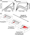 Figure 14.
Schematic diagram of throw profiles for abutting faults at different stages of development. Stage 1 is an isolated
Figure 14.
Schematic diagram of throw profiles for abutting faults at different stages of development. Stage 1 is an isolated ![]() fault
fault![]()
![]() profile
profile![]() . Stage 2 is an early-stage abutment with throw minima at the tips of the faults; Stage 3 is an intermediate stage with throw increasing at the abutting tip; and Stage 4 is a fully developed abutting
. Stage 2 is an early-stage abutment with throw minima at the tips of the faults; Stage 3 is an intermediate stage with throw increasing at the abutting tip; and Stage 4 is a fully developed abutting ![]() fault
fault![]() with a maximum throw at the abutting tip. Panels (A) and (B) represent abutting faults with an unrestricted and restricted tip, respectively. (C) Three-dimensional cartoon illustrating a developing abutting
with a maximum throw at the abutting tip. Panels (A) and (B) represent abutting faults with an unrestricted and restricted tip, respectively. (C) Three-dimensional cartoon illustrating a developing abutting ![]() fault
fault![]() shaded. The shading represents the displacement distribution of the abutting
shaded. The shading represents the displacement distribution of the abutting ![]() fault
fault![]() . See text for discussion.
. See text for discussion.
Trailing Faults
Although Figure 9 indicates that many long faults in the ![]() fault
fault![]() network are acting as isolated individual faults, increases and decreases often occur in some of their throw profiles. These usually coincide with abutments and interactions with other faults of the opposite
network are acting as isolated individual faults, increases and decreases often occur in some of their throw profiles. These usually coincide with abutments and interactions with other faults of the opposite ![]() fault
fault![]() set causing local reactivation of the pre-existing abutted-
set causing local reactivation of the pre-existing abutted-![]() fault
fault![]()
![]() plane
plane![]() (compare Figure 11). Sometimes a section of a
(compare Figure 11). Sometimes a section of a ![]() fault
fault![]()
![]() plane
plane![]() between two abutting faults is reactivated. This can be seen particularly well for longer west-northwest–trending faults the
between two abutting faults is reactivated. This can be seen particularly well for longer west-northwest–trending faults the ![]() fault
fault![]() planes for which show a change in displacement between the intersections with two abutting north-northeast–trending faults (Figure 15). This indicates trailing of displacement from the abutting faults onto the original pre-existing abutted
planes for which show a change in displacement between the intersections with two abutting north-northeast–trending faults (Figure 15). This indicates trailing of displacement from the abutting faults onto the original pre-existing abutted ![]() fault
fault![]() .
.
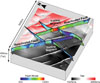 Figure 15.
Three-dimensional diagram of north-northeast–trending
Figure 15.
Three-dimensional diagram of north-northeast–trending ![]() fault
fault![]() planes that abut and locally reactivate west-northwest–trending
planes that abut and locally reactivate west-northwest–trending ![]() fault
fault![]() planes and form a trailing
planes and form a trailing ![]() fault
fault![]() segment that links two abutting faults. The distribution of throw is contoured onto each
segment that links two abutting faults. The distribution of throw is contoured onto each ![]() fault
fault![]()
![]() plane
plane![]() and shows increases in throw at the trailing
and shows increases in throw at the trailing ![]() fault
fault![]() segments. This example is taken from the SAG horizon. See Figure 3C for the locations of these faults within the
segments. This example is taken from the SAG horizon. See Figure 3C for the locations of these faults within the ![]() fault
fault![]() network. TWT = two-way time.
network. TWT = two-way time.
For example, the west-northwest–trending ![]() fault
fault![]() 207-SAG, seen in Figure 16, is abutted by two north-northeast–trending faults at intersections A (
207-SAG, seen in Figure 16, is abutted by two north-northeast–trending faults at intersections A (![]() fault
fault![]() 240-SAG) and B (
240-SAG) and B (![]() fault
fault![]() 121-SAG). The two abutting faults have very similar throw values near the points of intersection (Figure 16B), whereas the segment AB of the west-northwest–trending
121-SAG). The two abutting faults have very similar throw values near the points of intersection (Figure 16B), whereas the segment AB of the west-northwest–trending ![]() fault
fault![]() (
(![]() fault
fault![]() 207-SAG) shows a marked increase in accumulated throw between the two abutting faults (Figure 16A). A reconstruction of the original throw profiles (Figure 16) indicates that the increase in throw along segment AB (35–40 m [115–131 ft]) is broadly similar to the throw values of the two abutting faults at their points of intersection (35–40 m [115–131 ft]). This suggests that the movement of the two abutting north-northeast-faults (faults 240-SAG and 121-SAG) has reactivated segment AB producing a trailing-
207-SAG) shows a marked increase in accumulated throw between the two abutting faults (Figure 16A). A reconstruction of the original throw profiles (Figure 16) indicates that the increase in throw along segment AB (35–40 m [115–131 ft]) is broadly similar to the throw values of the two abutting faults at their points of intersection (35–40 m [115–131 ft]). This suggests that the movement of the two abutting north-northeast-faults (faults 240-SAG and 121-SAG) has reactivated segment AB producing a trailing-![]() fault
fault![]() segment. This links the two abutting faults to form a trailing
segment. This links the two abutting faults to form a trailing ![]() fault
fault![]() . The increase in throw along the trailing-
. The increase in throw along the trailing-![]() fault
fault![]() segment AB is because it shares the same kinematic motion sense (i.e., downthrown to the east) as the two abutting faults. Therefore, this may be regarded as a synthetic trailing interaction.
segment AB is because it shares the same kinematic motion sense (i.e., downthrown to the east) as the two abutting faults. Therefore, this may be regarded as a synthetic trailing interaction.
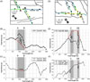 Figure 16.
![]() Fault
Fault![]() -throw profiles showing examples of trailing
-throw profiles showing examples of trailing ![]() fault
fault![]() interactions: (A), (B), and (C) show a synthetic trailing
interactions: (A), (B), and (C) show a synthetic trailing ![]() fault
fault![]() interaction in which two faults abut and reactivate a portion of another
interaction in which two faults abut and reactivate a portion of another ![]() fault
fault![]() that shares the same motion sense. (A) Plan-view map of the
that shares the same motion sense. (A) Plan-view map of the ![]() fault
fault![]() interaction. In this case,
interaction. In this case, ![]() fault
fault![]() 207 in (B) is reactivated between intersection points A and B, increasing in throw, because of the abutting interactions of faults 121 and 240 shown in (C); (D), (E), and (F) show an example of an antithetic trailing
207 in (B) is reactivated between intersection points A and B, increasing in throw, because of the abutting interactions of faults 121 and 240 shown in (C); (D), (E), and (F) show an example of an antithetic trailing ![]() fault
fault![]() in which faults abut and reactivate a portion of another
in which faults abut and reactivate a portion of another ![]() fault
fault![]() that has the opposite-motion sense. (D) Plan-view map of the
that has the opposite-motion sense. (D) Plan-view map of the ![]() fault
fault![]() interaction. In this case,
interaction. In this case, ![]() fault
fault![]() 199 in (E) is reactivated between intersection points C and E, decreasing in throw, because of interactions with abutting faults 5, 249, and 72 shown in (F). The dashed lines are an estimated reconstruction of the original
199 in (E) is reactivated between intersection points C and E, decreasing in throw, because of interactions with abutting faults 5, 249, and 72 shown in (F). The dashed lines are an estimated reconstruction of the original ![]() fault
fault![]() -throw profiles before interaction. See Figure 3C for the locations of these faults within the
-throw profiles before interaction. See Figure 3C for the locations of these faults within the ![]() fault
fault![]() network.
network.
In addition, examples of antithetic trailing interactions exist between the two ![]() fault
fault![]() sets (Figure 16D, E, F). These are produced when the trailing segment does not share the same motion sense as the abutting faults. For example,
sets (Figure 16D, E, F). These are produced when the trailing segment does not share the same motion sense as the abutting faults. For example, ![]() fault
fault![]() 199-SAG is a west-northwest–trending
199-SAG is a west-northwest–trending ![]() fault
fault![]() that is downthrown to the west, whereas the abutting faults (faults 240-SAG, 72-SAG, and 5-SAG) are all downthrown to the east (Figure 16F). As a result, marked drops occur in the throw
that is downthrown to the west, whereas the abutting faults (faults 240-SAG, 72-SAG, and 5-SAG) are all downthrown to the east (Figure 16F). As a result, marked drops occur in the throw ![]() profile
profile![]() of
of ![]() fault
fault![]() 199-SAG at intersection point A and between intersection points B and C. The reconstructed throw
199-SAG at intersection point A and between intersection points B and C. The reconstructed throw ![]() profile
profile![]() of
of ![]() fault
fault![]() 199-SAG (dashed line; Figure 16E) indicates that these decreases in throw match the throw values of the three abutting faults at the points of intersection. Furthermore, the throw profiles of the abutting faults are broadly coherent on either side of
199-SAG (dashed line; Figure 16E) indicates that these decreases in throw match the throw values of the three abutting faults at the points of intersection. Furthermore, the throw profiles of the abutting faults are broadly coherent on either side of ![]() fault
fault![]() 199-SAG (Figure 16E). This indicates that segment AC on
199-SAG (Figure 16E). This indicates that segment AC on ![]() fault
fault![]() 199-SAG inversely reactivated and interacted with the three abutting faults producing a kinematic and geometric link between them.
199-SAG inversely reactivated and interacted with the three abutting faults producing a kinematic and geometric link between them.
Thus, two types of trailing interactions occur between different ![]() fault
fault![]() sets. A synthetic trailing interaction produces a trailing
sets. A synthetic trailing interaction produces a trailing ![]() fault
fault![]() with segments that have the same motion sense (Figure 16). These cause an increase in throw along the trailing segment. Whereas, an antithetic trailing interaction involves abutting faults that have the opposite motion sense to the trailing segment causing inversion of the reactivated trailing segment and a decrease in throw (Figure 16).
with segments that have the same motion sense (Figure 16). These cause an increase in throw along the trailing segment. Whereas, an antithetic trailing interaction involves abutting faults that have the opposite motion sense to the trailing segment causing inversion of the reactivated trailing segment and a decrease in throw (Figure 16).
In summary, the trailing ![]() fault
fault![]() interactions involve faults sets that are at a high angle (i.e., orthogonal) to one another. As a result, the pre-existing
interactions involve faults sets that are at a high angle (i.e., orthogonal) to one another. As a result, the pre-existing ![]() fault
fault![]() is only locally reactivated and acts as a transfer
is only locally reactivated and acts as a transfer ![]() fault
fault![]() between the abutting faults, with the reactivated segment being analogous to a linking
between the abutting faults, with the reactivated segment being analogous to a linking ![]() fault
fault![]() that may breach a relay ramp between two parallel
that may breach a relay ramp between two parallel ![]() fault
fault![]() segments. This provides a kinematic link as well as a geometric link between the two abutting faults (Figure 15). Maerten (2000) describes similar trailing interactions between faults from the Chimney Rock
segments. This provides a kinematic link as well as a geometric link between the two abutting faults (Figure 15). Maerten (2000) describes similar trailing interactions between faults from the Chimney Rock ![]() fault
fault![]() array in central Utah. These include the Bluebell
array in central Utah. These include the Bluebell ![]() fault
fault![]() which has an increase in displacement on a segment between two abutting faults. The segment also has slickensides with different pitch orientations to the rest of the
which has an increase in displacement on a segment between two abutting faults. The segment also has slickensides with different pitch orientations to the rest of the ![]() fault
fault![]() , indicating reactivation and a kinematic link between the two abutting faults (Maerten, 2000).
, indicating reactivation and a kinematic link between the two abutting faults (Maerten, 2000).
EFFECTS OF PRE-EXISTING STRUCTURES AT DEPTH
Analysis of the ![]() fault
fault![]() network at Milne Point has shown that the deeper SAG horizon has higher
network at Milne Point has shown that the deeper SAG horizon has higher ![]() fault
fault![]() densities and accommodates larger strains in comparison with the KUP horizon. These changes are attributed to an increase in the number and size of the earlier west-northwest–trending faults as the later north-northeast–trending faults have similar density and strain values at each horizon (Table 1). We have suggested that the west-northwest–trending faults are influenced by the pre-existing underlying structural grain that trends northwest–southeast and bounds broad-scale horst and graben structures. This affects the largest faults within the network, which become steeper with depth (Figure 2), increase in throw in the SAG horizon (Figure 6), and are often oriented northwest–southeast matching the underlying structural grain (Figure 3).
densities and accommodates larger strains in comparison with the KUP horizon. These changes are attributed to an increase in the number and size of the earlier west-northwest–trending faults as the later north-northeast–trending faults have similar density and strain values at each horizon (Table 1). We have suggested that the west-northwest–trending faults are influenced by the pre-existing underlying structural grain that trends northwest–southeast and bounds broad-scale horst and graben structures. This affects the largest faults within the network, which become steeper with depth (Figure 2), increase in throw in the SAG horizon (Figure 6), and are often oriented northwest–southeast matching the underlying structural grain (Figure 3).
To investigate this influence further, Figure 17 shows the throw profiles for a group of four large west-northwest–trending faults (faults i, ii, iii, and iv) at the KUP and SAG horizons. All of these faults downthrow to the southwest, including smaller splay faults and breach faults in relays. In plan view, only faults ii (pink) and iii (orange) are geometrically linked, and these share relay ramps with ![]() fault
fault![]() i (blue) to the northwest and
i (blue) to the northwest and ![]() fault
fault![]() iv (turquoise) to the southeast (Figure 14). This suggests that these are interacting
iv (turquoise) to the southeast (Figure 14). This suggests that these are interacting ![]() fault
fault![]() segments at different stages of linkage.
segments at different stages of linkage.
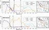 Figure 17.
![]() Fault
Fault![]() -throw profiles from (A) the KUP horizon and (B) the SAG horizon of four large west-northwest–trending faults (Faults i, ii, iii, and iv) that share relay ramps and interact with each other with some associated splay faults. The plots show variations in throw for each
-throw profiles from (A) the KUP horizon and (B) the SAG horizon of four large west-northwest–trending faults (Faults i, ii, iii, and iv) that share relay ramps and interact with each other with some associated splay faults. The plots show variations in throw for each ![]() fault
fault![]() along distance X, which increases to the east, indicating an increase in interaction, linkage, and a clockwise rotation with depth. To the right are plan-view maps of the interacting faults. See Figure 3C for the locations of these faults within the
along distance X, which increases to the east, indicating an increase in interaction, linkage, and a clockwise rotation with depth. To the right are plan-view maps of the interacting faults. See Figure 3C for the locations of these faults within the ![]() fault
fault![]() network.
network.
A comparison of the plan-view geometries of the four ![]() fault
fault![]() segments at each horizon indicates that faults i, iii, and iv are re-oriented further clockwise in the deeper SAG horizon and become aligned with the northwest–southeast structural grain (Figure 17). In addition, the relay ramps between each
segments at each horizon indicates that faults i, iii, and iv are re-oriented further clockwise in the deeper SAG horizon and become aligned with the northwest–southeast structural grain (Figure 17). In addition, the relay ramps between each ![]() fault
fault![]() segment decrease from ∼750 m (∼2461 ft) at the shallower KUP horizon to ∼250 m (∼820 ft) at the deeper SAG horizon (Figure 17). This indicates that the
segment decrease from ∼750 m (∼2461 ft) at the shallower KUP horizon to ∼250 m (∼820 ft) at the deeper SAG horizon (Figure 17). This indicates that the ![]() fault
fault![]() segments are becoming more geometrically linked with depth. The geometrical relationship between
segments are becoming more geometrically linked with depth. The geometrical relationship between ![]() fault
fault![]() iii and the other faults further supports this. In the KUP horizon,
iii and the other faults further supports this. In the KUP horizon, ![]() fault
fault![]() iii (orange) is linked to
iii (orange) is linked to ![]() fault
fault![]() ii (pink) by a breach
ii (pink) by a breach ![]() fault
fault![]() between intersection points A and B but becomes a throughgoing
between intersection points A and B but becomes a throughgoing ![]() fault
fault![]() in the SAG horizon that spans the distance between faults i (blue) and iv (turquoise), whereas
in the SAG horizon that spans the distance between faults i (blue) and iv (turquoise), whereas ![]() fault
fault![]() ii becomes a splay
ii becomes a splay ![]() fault
fault![]() at intersection point E (Figure 17). Furthermore, in the SAG horizon a breach
at intersection point E (Figure 17). Furthermore, in the SAG horizon a breach ![]() fault
fault![]() forms at intersection point D in the relay between faults i and iii (Figure 17B).
forms at intersection point D in the relay between faults i and iii (Figure 17B).
The throw profiles of each ![]() fault
fault![]() indicate that they accumulate more throw with depth and become more developed. For example, in the KUP horizon
indicate that they accumulate more throw with depth and become more developed. For example, in the KUP horizon ![]() fault
fault![]() iii (orange) has an incongruent
iii (orange) has an incongruent ![]() fault
fault![]()
![]() profile
profile![]() with a splay
with a splay ![]() fault
fault![]() (intersection point C) and a breach
(intersection point C) and a breach ![]() fault
fault![]() (intersection point B) causing large step-like variations in its throw
(intersection point B) causing large step-like variations in its throw ![]() profile
profile![]() (Figure 17A). This matches the splay faults described in Figure 10. However, in the deeper SAG horizon,
(Figure 17A). This matches the splay faults described in Figure 10. However, in the deeper SAG horizon, ![]() fault
fault![]() iii has a more congruent throw
iii has a more congruent throw ![]() profile
profile![]() along its strike (Figure 17B), indicating that it has a coherent
along its strike (Figure 17B), indicating that it has a coherent ![]() fault
fault![]()
![]() plane
plane![]() . The throw profiles also indicate that the faults are more kinematically linked in the SAG horizon. For example, the throw
. The throw profiles also indicate that the faults are more kinematically linked in the SAG horizon. For example, the throw ![]() profile
profile![]() of
of ![]() fault
fault![]() iv (turquoise) has a symmetrical throw
iv (turquoise) has a symmetrical throw ![]() profile
profile![]() at the KUP horizon (Figure 17A) but an asymmetrical throw
at the KUP horizon (Figure 17A) but an asymmetrical throw ![]() profile
profile![]() in the SAG horizon with a very steep throw gradient at its northwest tip, indicating interaction with
in the SAG horizon with a very steep throw gradient at its northwest tip, indicating interaction with ![]() fault
fault![]() iii (Figure 17B).
iii (Figure 17B).
Overall, Figure 17 further supports that the development of west-northwest–trending faults was influenced by deeper pre-existing structures. The effect of these underlying structures is characterized by several changes with depth:
1. Clockwise rotation of west-northwest–trending faults with depth as they align themselves with the underlying structural grain (Figure 17);
2. Increase in ![]() fault
fault![]() dip of larger west-northwest–trending faults (Figures 2, 5);
dip of larger west-northwest–trending faults (Figures 2, 5);
3. Increase in throw and strain localization onto west-northwest–trending faults (Table 1);
4. Better linkage between large west-northwest–trending faults (Figure 17).
Reactivation of pre-existing structures can often produce and affect new ![]() fault
fault![]() sets in the overlying stratigraphy (Bailey et al., 2005; Frankowicz and McClay, 2010). For example, Bailey et al. (2005) see similar changes in the spatial development of two normal-
sets in the overlying stratigraphy (Bailey et al., 2005; Frankowicz and McClay, 2010). For example, Bailey et al. (2005) see similar changes in the spatial development of two normal-![]() fault
fault![]() sets in the East Pennines Coalfield (United Kingdom) caused by reactivation of underlying basement faults causing strain localization onto one
sets in the East Pennines Coalfield (United Kingdom) caused by reactivation of underlying basement faults causing strain localization onto one ![]() fault
fault![]() set.
set.
As the west-northwest–trending faults are obliquely oriented to the northwest-trending underlying structural grain, it is possible that these were driven by left-lateral transtension along the previous structures. This is supported by the strain orientation of the west-northwest-trending ![]() fault
fault![]() set, the steepening of the larger faults with depth, and the splaying and rotation of faults into the northwest-trending structural grain, which resembles the organization of faults in upward-splaying flower structures and bifurcating up-tips above left-lateral strike-slip faults (compare McGrath and Davison, 1995; Kim et al., 2004). Furthermore, Giba et al. (2012) show similar characteristics for an obliquely reactivated normal
set, the steepening of the larger faults with depth, and the splaying and rotation of faults into the northwest-trending structural grain, which resembles the organization of faults in upward-splaying flower structures and bifurcating up-tips above left-lateral strike-slip faults (compare McGrath and Davison, 1995; Kim et al., 2004). Furthermore, Giba et al. (2012) show similar characteristics for an obliquely reactivated normal ![]() fault
fault![]() in the Taranaki Basin, New Zealand, with
in the Taranaki Basin, New Zealand, with ![]() fault
fault![]() splays propagating upward from the reactivated
splays propagating upward from the reactivated ![]() fault
fault![]() and rotating to align with the regional stress field.
and rotating to align with the regional stress field.
SUMMARY AND CONCLUSIONS
A normal-![]() fault
fault![]() network from onshore Milne Point, Alaska has been analyzed using 3-D seismic reflection data. The network comprises north-northeast–trending and west-northwest–trending
network from onshore Milne Point, Alaska has been analyzed using 3-D seismic reflection data. The network comprises north-northeast–trending and west-northwest–trending ![]() fault
fault![]() sets, which were analyzed at two stratigraphic horizons: the Kuparuk River and the Sag River formations, which are both hydrocarbon reservoir formations. Analysis shows that the following.
sets, which were analyzed at two stratigraphic horizons: the Kuparuk River and the Sag River formations, which are both hydrocarbon reservoir formations. Analysis shows that the following.
1. Both ![]() fault
fault![]() orientations are different generations of faulting. We suggest a Jurassic age for the west-northwest–trending faults and a Cenozoic age for the north-northeast–trending faults. It is also probable that there has been later reactivation of parts of the west-northwest–trending faults both during formation of the north-northeast–trending faults and subsequent stress.
orientations are different generations of faulting. We suggest a Jurassic age for the west-northwest–trending faults and a Cenozoic age for the north-northeast–trending faults. It is also probable that there has been later reactivation of parts of the west-northwest–trending faults both during formation of the north-northeast–trending faults and subsequent stress.
2. The north-northeast–trending faults generally dip to the southeast producing a strain with a maximum extension orientation of ∼N103°E. These are consistently developed in both horizons with similar ![]() fault
fault![]() densities,
densities, ![]() fault
fault![]() sizes, and strains. In contrast, the majority of west-northwest–trending faults dip to the southwest and have a strain tensor with a maximum extension orientation of ∼N30°E. They show variation with depth increasing in size, number, and density, hence accommodating greater strains. The overall strain accommodated by the
sizes, and strains. In contrast, the majority of west-northwest–trending faults dip to the southwest and have a strain tensor with a maximum extension orientation of ∼N30°E. They show variation with depth increasing in size, number, and density, hence accommodating greater strains. The overall strain accommodated by the ![]() fault
fault![]() network is a superposition of the two strain tensors.
network is a superposition of the two strain tensors.
Mapping variations in throw along ![]() fault
fault![]() planes and around intersections lines (branch lines) allowed the identification of numerous interactions within the
planes and around intersections lines (branch lines) allowed the identification of numerous interactions within the ![]() fault
fault![]() network. Faults can be divided into isolated, abutting, and splaying faults. In general, abutments and cross-cutting faults involve faults from different
network. Faults can be divided into isolated, abutting, and splaying faults. In general, abutments and cross-cutting faults involve faults from different ![]() fault
fault![]() sets, whereas splay faults are from the same
sets, whereas splay faults are from the same ![]() fault
fault![]() set. The different interactions can be characterized by their throw distributions along
set. The different interactions can be characterized by their throw distributions along ![]() fault
fault![]() planes (summarized in Table 3):
planes (summarized in Table 3):
3. Isolated faults produce symmetrical or asymmetrical ![]() fault
fault![]() profiles depending on the degree of restriction at
profiles depending on the degree of restriction at ![]() fault
fault![]() tips, which can be identified by high-throw gradient at the restricted tip.
tips, which can be identified by high-throw gradient at the restricted tip.
4. Splay faults have a throw maximum at the line of intersection and steadily decrease in throw toward their tip. They accommodate decreases in throw along a larger main ![]() fault
fault![]() .
.
5. Abutting faults form a range of throw profiles depending on the timing of abutment during ![]() fault
fault![]() development. There are two main groups: early-stage abutting faults with throw minima at the abutting and isolated tips and late-stage abutting faults that have grown and accumulated a throw maximum at the abutting tip.
development. There are two main groups: early-stage abutting faults with throw minima at the abutting and isolated tips and late-stage abutting faults that have grown and accumulated a throw maximum at the abutting tip.
Developing faults within the network also interact with pre-existing structures. These can be oriented at either a high angle or a low angle to each other and have different characteristics (summarized in Table 3):
6. Abutting faults form at high angles to the pre-existing ![]() fault
fault![]() . As a result, when they grow and accumulate displacement after initial abutment, they locally reactivate the pre-existing
. As a result, when they grow and accumulate displacement after initial abutment, they locally reactivate the pre-existing ![]() fault
fault![]() through the transfer of displacement. This can produce a trailing
through the transfer of displacement. This can produce a trailing ![]() fault
fault![]() that links two abutting faults through the reactivated segment of the pre-existing
that links two abutting faults through the reactivated segment of the pre-existing ![]() fault
fault![]() . The motion sense of the trailing
. The motion sense of the trailing ![]() fault
fault![]() can either be synthetic or antithetic to the reactivated pre-existing
can either be synthetic or antithetic to the reactivated pre-existing ![]() fault
fault![]() producing an increase or decrease in throw, respectively.
producing an increase or decrease in throw, respectively.
7. The west-northwest–trending faults have interacted with the similarly oriented underlying northwest–southeast structural grain. This has resulted in reactivation of these pre-existing structures and has influenced the development of the west-northwest–trending faults. These influences are characterized by increases in dip and throw on several faults, strain localization, clockwise rotation of faults, and an increase in linkage maturity.
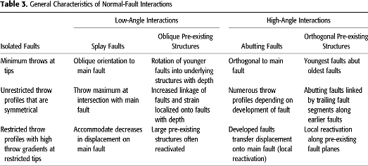
Overall, this paper provides a robust example of a network analysis applied to a normal-![]() fault
fault![]() network with cross-cutting relationships and multiple generations of faulting. Using throw distributions has identified and characterized numerous
network with cross-cutting relationships and multiple generations of faulting. Using throw distributions has identified and characterized numerous ![]() fault
fault![]() interactions as well as the influence of pre-existing structures on network development. It has also characterized different types of reactivation (i.e., local and regional) within
interactions as well as the influence of pre-existing structures on network development. It has also characterized different types of reactivation (i.e., local and regional) within ![]() fault
fault![]() networks. Identification of such interactions is important as it furthers our understanding of the kinematic behavior of faults within a
networks. Identification of such interactions is important as it furthers our understanding of the kinematic behavior of faults within a ![]() fault
fault![]() network.
network.
The geometry of the two generations of faulting means that the two reservoir horizons are at least geometrically compartmentalized by the faults. Therefore, this study has important implications for hydrocarbon exploration in northern Alaska. The identification of areas of local reactivation along ![]() fault
fault![]() planes, caused by abutting faults or trailing faults, could be particularly useful as this may produce an increased amount of
planes, caused by abutting faults or trailing faults, could be particularly useful as this may produce an increased amount of ![]() fault
fault![]() damage around intersection lines. Small faults and fractures associated with such damage could provide a fluid pathway across a previously sealing
damage around intersection lines. Small faults and fractures associated with such damage could provide a fluid pathway across a previously sealing ![]() fault
fault![]()
![]() plane
plane![]() . Hence, this could affect reservoir connectivity and/or provide communication between compartments. Therefore, being able to identify such interactions may influence the location of boreholes/wells into a compartmentalized reservoir.
. Hence, this could affect reservoir connectivity and/or provide communication between compartments. Therefore, being able to identify such interactions may influence the location of boreholes/wells into a compartmentalized reservoir.
REFERENCES CITED
Aydin, A., 2000. Fractures, faults, and hydrocarbon entrapment, migration and flow: Marine and Petroleum Geology, v. 17, no. 7, p. 797–814, doi: 10.1016/S0264-8172(00)00020-9.
Bailey, W. R., J. J. Walsh, and T. Manzocchi, 2005, ![]() Fault
Fault![]() populations, strain distribution and basement
populations, strain distribution and basement ![]() fault
fault![]() reactivation in the East Pennines Coalfield, UK: Journal of Structural Geology, v. 27, no. 5, p. 913–928, doi: 10.1016/j.jsg.2004.10.014.
reactivation in the East Pennines Coalfield, UK: Journal of Structural Geology, v. 27, no. 5, p. 913–928, doi: 10.1016/j.jsg.2004.10.014.
Bird, K. J., 1999, Geographic, and geologic setting, in The Oil and Gas Resource Potential of the 1002 Area, Arctic National Wildlife Refuge, Alaska, by ANWR Assessment Team, U.S. Geological Survey Open File Report 98-34: U.S. Geological Survey, Chapter 66, 51 p.
Boswell, R., K. Rose, T. S. Collett, M. Lee, W. Winters, K. A. Lewis, and W. Agena, 2011, Geologic controls on gas hydrate occurrence in the Mount Elbert prospect, Alaska North Slope: Marine and Petroleum Geology, v. 28, no. 2, p. 589–607, doi: 10.1016/j.marpetgeo.2009.12.004.
Bouvier, J., C. Kaars-Sijpesteijn, D. Kluesner, C. Onyejekwe, and R. van der Pal, 1989, Three-dimensional seismic interpretation and ![]() fault
fault![]() sealing investigations, Nun River Field, Nigeria: AAPG Bulletin, v. 73, no. 11, p. 1397–1414.
sealing investigations, Nun River Field, Nigeria: AAPG Bulletin, v. 73, no. 11, p. 1397–1414.
Carman, G., and P. Hardwick, 1983, Geology and regional setting of Kuparuk oil field, Alaska: AAPG Bulletin, v. 67, no. 6, p. 1014–1031.
Collett, T. S., 1993, Natural gas hydrates of the Prudhoe Bay and Kuparuk River area, North Slope, Alaska: AAPG Bulletin, v. 77, no. 5, p. 793–812.
Collett, T. S., M. W. Lee, W. F. Agena, J. J. Miller, K. A. Lewis, M. V. Zyrianova, R. Boswell, and T. L. Inks, 2011, Permafrost-associated natural gas hydrate occurrences on the Alaska North Slope: Marine and Petroleum Geology, v. 28, no. 2, p. 279–294, doi: 10.1016/j.marpetgeo.2009.12.001.
Davatzes, N. C., A. Aydin, and P. Eichhubl, 2003, Overprinting faulting mechanisms during the development of multiple ![]() fault
fault![]() sets in sandstone, Chimney Rock
sets in sandstone, Chimney Rock ![]() fault
fault![]() array, Utah, USA: Tectonophysics, v. 363, no. 1–2, p. 1–18, doi: 10.1016/S0040-1951(02)00647-9.
array, Utah, USA: Tectonophysics, v. 363, no. 1–2, p. 1–18, doi: 10.1016/S0040-1951(02)00647-9.
Dzou, L. I., 2010, Kuparuk oil field, Alaska, a mixture of Kekiktuk gas condensate and Shublik oil: AAPG Bulletin, v. 94, no. 11, p. 1761–1778, doi: 10.1306/06301009167.
Ferrill, D. A., and A. P. Morris, 2001, Displacement gradient and deformation in normal ![]() fault
fault![]() systems: Journal of Structural Geology, v. 23, p. 619–638, doi: 10.1016/S0191-8141(00)00139-5.
systems: Journal of Structural Geology, v. 23, p. 619–638, doi: 10.1016/S0191-8141(00)00139-5.
Ferrill, D. A., A. P. Morris, and R. N. McGinnis, 2009, Crossing conjugate normal faults in field exposures and seismic data: AAPG Bulletin, v. 93, no. 11, p. 1471–1488, doi: 10.1306/06250909039.
Fossen, H., T. E. S. Johansen, J. Hesthammer, and A. Rotevatn, 2005, ![]() Fault
Fault![]() interaction in porous sandstone and implications for reservoir management: Examples from southern Utah: AAPG Bulletin, v. 89, no. 12, p. 1593–1606, doi: 10.1306/07290505041.
interaction in porous sandstone and implications for reservoir management: Examples from southern Utah: AAPG Bulletin, v. 89, no. 12, p. 1593–1606, doi: 10.1306/07290505041.
Frankowicz, E., and K. R. McClay, 2010, Extensional ![]() fault
fault![]() segmentation and linkage, Bonaparte Basin, outer North West Shelf, Australia: AAPG Bulletin, v. 94, no. 7, p. 977–1010, doi: 10.1306/01051009120.
segmentation and linkage, Bonaparte Basin, outer North West Shelf, Australia: AAPG Bulletin, v. 94, no. 7, p. 977–1010, doi: 10.1306/01051009120.
Gartrell, A., W. R. Bailey, and M. Brincat, 2006, A new model for assessing trap integrity and oil preservation risks associated with postrift ![]() fault
fault![]() reactivation in the Timor Sea: AAPG Bulletin, v. 90, no. 12, p. 1921–1944, doi: 10.1306/06200605195.
reactivation in the Timor Sea: AAPG Bulletin, v. 90, no. 12, p. 1921–1944, doi: 10.1306/06200605195.
Giba, M., J. J. Walsh, and A. Nicol, 2012, Segmentation and growth of an obliquely reactivated normal ![]() fault
fault![]() : Journal of Structural Geology, v. 39, p. 253–267, doi: 10.1016/j.jsg.2012.01.004.
: Journal of Structural Geology, v. 39, p. 253–267, doi: 10.1016/j.jsg.2012.01.004.
Goteti, R., G. Mitra, A. Becene, A. Sussman, and C. Lewis, 2013, Three-dimensional finite-element modeling of ![]() fault
fault![]() interactions in rift-scale normal
interactions in rift-scale normal ![]() fault
fault![]() systems: Implications for the late Cenozoic Rio Grande rift of north central New Mexico, in M. R. Hudson, V. J. S. Grauch, eds., New Perspectives on Rio Grande Rift Basins: From Tectonics to Groundwater: Geological Society of America Special Paper 494, p. 157–184, doi: 10.1130/2013.2494(07).
systems: Implications for the late Cenozoic Rio Grande rift of north central New Mexico, in M. R. Hudson, V. J. S. Grauch, eds., New Perspectives on Rio Grande Rift Basins: From Tectonics to Groundwater: Geological Society of America Special Paper 494, p. 157–184, doi: 10.1130/2013.2494(07).
Heidbach, O., M. Tingay, A. Barth, J. Reinecker, D. Kurfeß, and B. Müller, 2010, Global crustal stress pattern based on the World Stress Map database release 2008: Tectonophysics, v. 482, no. 1–4, p. 3–15, doi: 10.1016/j.tecto.2009.07.023.
Hubbard, R., S. Edrich, and R. P. Rattey, 1987, Geologic evolution, and hydrocarbon habitat of the “Arctic Alaska Microplate”: Marine and Petroleum Geology, v. 4, no. 1, p. 2–34, doi: 10.1016/0264-8172(87)90019-5.
Imber, J., G. W. Tuckwell, C. Childs, J. J. Walsh, T. Manzocchi, A. E. Heath, C. G. Bonson, and J. Strand, 2004, Three-dimensional distinct element modeling of relay growth and breaching along normal faults: Journal of Structural Geology, v. 26, p. 1897–1911, doi: 10.1016/j.jsg.2004.02.010.
Jolley, S. J., Q. J. Fisher, and R. B. Ainsworth, 2010, Reservoir compartmentalization: An introduction. Geological Society: London, Special Publications, v. 347, p. 1–8, doi: 10.1144/SP347.1.
Kim, Y.-S., J. R. Andrews, and D. J. Sanderson, 2001, Reactivated strike–slip faults: Examples from north Cornwall, UK: Tectonophysics, v. 340, no. 3–4, p. 173–194, doi 10.1016/S0040-1951(01)00146-9.
Kim, Y.-S., D. C. Peacock, and D. J. Sanderson, 2004, ![]() Fault
Fault![]() damage zones: Journal of Structural Geology, v. 26, no. 3, p. 503–517, doi: 10.1016/j.jsg.2003.08.002.
damage zones: Journal of Structural Geology, v. 26, no. 3, p. 503–517, doi: 10.1016/j.jsg.2003.08.002.
Leveille, G., R. Knipe, C. More, D. Ellis, G. Dudley, G. Jones, Q. J. Fisher, and G. Allinson, 1997, Compartmentalization of Rotliegendes gas reservoirs by sealing faults, Jupiter Fields area, southern North Sea: Geological Society: London, Special Publications, v. 123, p. 87–104, doi: 10.1144/GSL.SP.1997.123.01.06.
Lorenson, T. D., T. S. Collett, and R. B. Hunter, 2011, Gas geochemistry of the Mount Elbert Gas Hydrate Stratigraphic Test Well, Alaska North Slope: Implications for gas hydrate exploration in the Arctic: Marine and Petroleum Geology, v. 28, no. 2, p. 343–360, doi: 10.1016/j.marpetgeo.2010.02.007.
Maerten, L., 2000, Variation in slip on intersecting normal faults-Implications for paleostress inversion: Journal of Geophysical Research, v. 105, no. B11, p. 25553–25565, doi: 10.1029/2000JB900264.
Maerten, L., D. Pollard, and F. Maerten, 2001, Digital mapping of three-dimensional structures of the Chimney Rock ![]() fault
fault![]() system, central Utah: Journal of Structural Geology, v. 23, no. 4, p. 585–592, doi: 10.1016/S0191-8141(00)00142-5.
system, central Utah: Journal of Structural Geology, v. 23, no. 4, p. 585–592, doi: 10.1016/S0191-8141(00)00142-5.
Maerten, L., E. J. M. Willemse, D. D. Pollard, and K. Rawnsley, 1999, Slip distributions on intersecting normal faults: Journal of Structural Geology, v. 21, no. 3, p. 259–272, doi: 10.1016/S0191-8141(98)00122-9.
Manighetti, I., G. King, Y. Gaudemer, and C. Scholz, 2001, Slip accumulation and lateral propagation of active normal faults in Afar: Journal of Geophysical Research, v. 106, no. B7, p. 13667–13696, doi: 10.1029/2000JB900454.
Masterson, W., L. Dzou, and A. Holba, 2001, Evidence for biodegradation and evaporative fractionation in West Sak, Kuparuk and Prudhoe Bay field areas, North Slope, Alaska: Organic Geochemistry, v. 32, no. 3, p. 411–441, doi: 10.1016/S0146-6380(00)00187-X.
McGrath, A., and I. Davison, 1995, Damage zone geometry around ![]() fault
fault![]() tips: Journal of Structural Geology, v. 17, no. 7, p. 1011–1024, doi: 10.1016/0191-8141(94)00116-H.
tips: Journal of Structural Geology, v. 17, no. 7, p. 1011–1024, doi: 10.1016/0191-8141(94)00116-H.
Muraoka, H., and H. Kamata, 1983, Displacement distribution along minor ![]() fault
fault![]() traces: Journal of Structural Geology, v. 5, no. 5, p. 483–495, doi: 10.1016/0191-8141(83)90054-8.
traces: Journal of Structural Geology, v. 5, no. 5, p. 483–495, doi: 10.1016/0191-8141(83)90054-8.
Nicol, A., J. Walsh, J. Watterson, and P. Bretan, 1995, Three-dimensional geometry and growth of conjugate normal faults: Journal of Structural Geology, v. 17, no. 6, p. 847–862, doi: 10.1016/0191-8141(94)00109-D.
Nicol, A., J. Watterson, J. Walsh, and C. Childs, 1996, The shapes, major axis orientations and displacement patterns of ![]() fault
fault![]() surfaces: Journal of Structural Geology, v. 18, no. 2/3, p. 235–248, doi: 10.1016/S0191-8141(96)80047-2.
surfaces: Journal of Structural Geology, v. 18, no. 2/3, p. 235–248, doi: 10.1016/S0191-8141(96)80047-2.
Nicol, A., J. J. Walsh, P. Villamor, H. Seebeck, and K. R. Berryman, 2010, Normal ![]() fault
fault![]() interactions, paleoearthquakes and growth in an active rift: Journal of Structural Geology, v. 32, no. 8, p. 1101–1113, doi: 10.1016/j.jsg.2010.06.018.
interactions, paleoearthquakes and growth in an active rift: Journal of Structural Geology, v. 32, no. 8, p. 1101–1113, doi: 10.1016/j.jsg.2010.06.018.
Ning, S. X., and P. L. McGuire, 2004, Improved Oil Recovery in Under-Saturated Reservoirs Using the US-WAG Process: SPE 89353, 6 p.
Nixon, C. W., D. J. Sanderson, and J. M. Bull, 2011, Deformation within a strike-slip ![]() fault
fault![]() network at Westward Ho!, Devon UK: Domino vs conjugate faulting: Journal of Structural Geology, v. 33, no. 5, p. 833–843, doi: 10.1016/j.jsg.2011.03.009.
network at Westward Ho!, Devon UK: Domino vs conjugate faulting: Journal of Structural Geology, v. 33, no. 5, p. 833–843, doi: 10.1016/j.jsg.2011.03.009.
Peacock, D. C. P., and D. J. Sanderson, 1991, Displacements, segment linkage and relay zones in normal ![]() fault
fault![]() zones: Journal of Structural Geology, v. 13, no. 6, p. 721–733, doi: 10.1016/0191-8141(91)90033-F.
zones: Journal of Structural Geology, v. 13, no. 6, p. 721–733, doi: 10.1016/0191-8141(91)90033-F.
Peacock, D. C. P., and D. J. Sanderson, 1993, Estimating strain from ![]() fault
fault![]() slip using a line sample: Journal of Structural Geology, v. 15, no. 12, p. 1513–1516, doi: 10.1016/0191-8141(93)90011-X.
slip using a line sample: Journal of Structural Geology, v. 15, no. 12, p. 1513–1516, doi: 10.1016/0191-8141(93)90011-X.
Peacock, D. C. P., and D. J. Sanderson, 1996, Effects of propagation rate on displacement variations along faults: Journal of Structural Geology. v. 18, no. 2/3, p. 311–320, doi: 10.1016/S0191-8141(96)80052-6.
Pollard, D., and P. Segall, 1987, Theoretical displacements and stresses near fractures in rock: With applications to faults, joints, veins, dikes, and solution surfaces, in B. Atkinson, ed., Fracture Mechanics of Rock: Academic Press, New York, pp. 277–349.
Schlagenhauf, A., I. Manighetti, J. Malavieille, and S. Dominguez, 2008, Incremental growth of normal faults: Insights from a laser-equipped analog experiment: Earth and Planetary Science Letters, v. 273, no. 3–4, p. 299–311, doi: 10.1016/j.epsl.2008.06.042.
Segall, P., and D. Pollard, 1983, Nucleation and growth of strike slip faults in granite: Journal of Geophysical Research, v. 88, no. B1, p. 555–568, doi: 10.1029/JB088iB01p00555.
Soliva, R., and A. Benedicto, 2004, A linkage criterion for segmented normal faults: Journal of Structural Geology, v. 26, no. 12, p. 2251–2267, doi: 10.1016/j.jsg.2004.06.008.
Soliva, R., and A. Benedicto, 2005, Geometry, scaling relations and spacing of vertically restricted normal faults: Journal of Structural Geology, v. 27, no. 2, p. 317–325, doi: 10.1016/j.jsg.2004.08.010.
Walsh, J., W. Bailey, C. Childs, A. Nicol, and C. Bonson, 2003, Formation of segmented normal faults: a 3-D perspective: Journal of Structural Geology, v. 25, no. 8, p. 1251–1262, doi: 10.1016/S0191-8141(02)00161-X.
Zhao, G., and A. Johnson, 1991, Sequential and incremental formation of conjugate sets of faults. Journal of Structural Geology, v. 13, no. 8, p. 887–895, doi: 10.1016/0191-8141(91)90084-V.
Zoback, M. L., 1992, First- and second-order patterns of stress in the lithosphere: The World Stress Map Project: Journal of Geophysical Research, v. 97, no. B8, p. 11703–11728, doi: 10.1029/92JB00132.
AUTHORS
Casey Nixon received his B.Sc. Honors degree in geology from the University of Edinburgh and his Ph.D. in structural geology from the University of Southampton. He is presently working as a post-doctoral research and teaching fellow at the University of Southampton. His current research interests are ![]() fault
fault![]() and fracture network analysis, basin dynamics, active rifting, and seismic hazard assessment.
and fracture network analysis, basin dynamics, active rifting, and seismic hazard assessment.
David Sanderson is professor of tectonics and geomechanics at the University of Southampton and a consultant to BP. His main research interests are faulting, fracturing, and fluid flow, with applications in the hydrocarbon, mineral, and engineering industries. He has published over 130 scientific articles and a recent book on distinct element modeling of deformation and fluid flow in fractured rock.
Stephen Dee is a senior structural geologist at BP, working in the Integrated Subsurface Description and Modelling team and consulting on structural and geomechanics projects. He has a Ph.D. from the University of Southampton and specializes in ![]() fault
fault![]() and fracture interpretation, geomechanical modeling, and seal analysis.
and fracture interpretation, geomechanical modeling, and seal analysis.
Jonathan Bull is professor of geophysics at the University of Southampton with main research interests in marine seismology and structural geology. He has published more than 70 peer-reviewed publications and has developed and licensed technology related to 3-D marine imaging.
Robert Humphreys received his M.A. degree in natural sciences from Cambridge University, and Ph.D. in structural geology from Cardiff University (UK). He has worked in exploration, production and structural geology technology teams for BP and is currently assisting Alaskan North Slope development. One of his particular interests is developing structural guidelines for seismic interpretation.
Mark Swanson received his M.S. degree in geology from the University of Toledo, Ohio, and has been further trained in geophysics. He has worked in both exploration and production and is presently working on the Milne Point Reservoir Management Team trying to better understand the compartmentalization of this highly faulted field.
ACKNOWLEDGEMENTS
The research presented in this paper was completed as part of a Ph.D. by C. W. Nixon supported financially from a NERC case studentship (NE/H524922/1) with BP. We thank the Milne Point Reservoir Management Team, BP Exploration (Alaska) for provision of the 3-D seismic reflection data used in this article. In particular, we thank Kip Cerveny (team leader, Milne Point Reservoir Management Team) and Rebecca Bailey (geologist, Milne Point) for their input and support. We would also like to thank the Integrated Subsurface Description and Modelling team, BP Exploration (Sunbury) for their logistical and technical support throughout.
The AAPG Editor thanks Senior Associate Editor Richard H. Groshong and the following reviewers for their work on this paper: Daniel Ciulavu, J. Steven Davis, and an anonymous reviewer.
EDITOR’S NOTE
Color versions of Figures 1, 14, and 16 may be seen in the online Open Access version of this paper.