INTRODUCTION

Natural gas plays an essential role in the possible transitions to clean energy. Today, natural gas fulfills one-fourth of the global primary power demand (BP, 2020), and its importance to the global power supply mix is predicted to only increase in the next two decades. In the United States, natural gas provides one-third of the total primary power demand (Energy Information Administration, 2020b). In mid-2020, the United States produced nearly 110 BCF of natural gas per day, which is almost twice the production rate of 15 yr ago (Enverus, 2021). This significant increase in natural gas output in the United States has only been possible with the “unconventional resource revolution” over the last two decades, during which operators have learned how to produce gas from the extremely low-permeability—unconventional—mudrock or so-called shale formations by advancing horizontal drilling and hydraulic fracturing technologies. Today, the eight major shale plays in the United States are responsible for nearly 70% of the total natural gas output. The Marcellus Shale, the largest gas shale play in North America, contributes one-third of the total United States shale gas production, producing more than 25 BCF of natural gas per day. As of the writing of this paper, the Marcellus has produced 50 trillion SCF (TSCF) of natural gas, equivalent to 8.3 billion bbl of oil.

Despite the key role of the Marcellus in securing national power demand, a significant disparity exists in the predictions of the total amount of technically recoverable gas contained in the Marcellus. A study by the Bureau of Economic Geology (BEG) at The University of Texas at Austin (Ikonnikova et al., 2018), predicted the technically recoverable resources (TRRs) of the Marcellus to be 560 TSCF. The US Department of Energy’s Energy Information Administration (EIA) recently published a prediction of 310.6 TSCF of technically recoverable gas (Energy Information Administration, 2020a). Lastly, the US Geological Survey (USGS) estimated only 96.5 TSCF of total undiscovered resources in the Marcellus. This divergence of total producible resource predictions in the Marcellus shows just how difficult and uncertain the resource assessment in unconventional reservoirs is. Conventional reservoirs can be evaluated by identifying their structures, traps, and water–gas contacts. Assessment of recoverable resources in unconventional reservoirs is highly uncertain and unfeasible with use of the traditional volumetric methods (Schmoker, 2002; Haskett and Brown, 2005; Cipolla et al., 2011; Zou, 2017). In unconventional reservoirs, hydrocarbon accumulations exist continuously and span huge areas of shale or tight carbonate–sandstone formations. However, because of the extremely limited reservoir connectivity, thousands of horizontal hydraulically fractured wells must be drilled to achieve a desirable rate of production. Therefore, the risk of hydrocarbon finding, which is key to assessing conventional reservoirs, becomes insignificant relative to the risk of commerciality (Fulford, 2016).

In many unconventional plays, better-producing zones are concentrated in smaller geographic and geologic zones that are often called “sweet spots” (Hughes, 2013). Another factor that compounds the uncertainty of unconventional resource assessment is the advancement of completion technologies (Weijermars, 2015). Modern wells with new completions generally outperform vintage wells in the same reservoir, but with traditional completion systems. These new wells are completed with intensive hydraulic fracturing treatments (more of larger hydraulic fractures).

In this paper, we pursue our tested integrated approach, which minimizes the uncertainty of fieldwide resource assessment in the Marcellus. Following USGS (Higley et al., 2019), we focus only on the Middle Devonian Marcellus layer. There may be additional potential production coming from adjacent formations, such as the Upper Devonian Shale. However, as of January 2021, there were only 399 wells producing from the Upper Devonian that produced negligible gas in comparison with the 15,000+ wells drilled in the Middle Devonian Marcellus (see, for example, Milici and Swezey, 2014, for a full stratigraphic cross section/type section of the Appalachian Basin). By including fundamentals of shale geology, advancement of well completion technologies, physics of natural gas production from the hydraulically fractured shales, and economics of drilling projects, our approach is different from the volumetric approach of USGS (Higley et al., 2019). According to the classification of the resource assessment approaches for unconventional formations (Schmoker, 2002), our method belongs to his second category that relies heavily on production performance of existing wells, instead of the highly uncertain volumetric estimates in category one.

First, we divide the Marcellus Shale play into several spatiotemporal well cohorts in which gas production is statistically uniform. Second, for each cohort, we construct a hybrid data-driven and physics-based well prototype based on the generalized extreme value (GEV) statistics (Fréchet, 1927; Weibull et al., 1951; Gumbel, 1954) and on physical scaling (Patzek et al., 2013, 2014, 2017; Eftekhari et al., 2020; Saputra et al., 2020, 2021a; Saputra, 2021). We have previously introduced the hybrid GEV + physical scaling method in Patzek (2019), Patzek et al. (2019), and Saputra et al. (2019), in which we constructed well prototypes for the Barnett Formation and Bakken Formation shales. To check whether we have the robust well prototypes that best represent at times more than 1000 wells per cohort, we replace production from each existing well with its corresponding well prototype. Since the summation of production from the time-shifted well prototypes matches the total historical field rate, the extrapolated future production serves as our base or do-nothing forecast, which gives a robust estimated ultimate recovery (EUR) from all of the existing wells in the Marcellus.

To obtain the fieldwide EUR, we also calculate the most plausible numbers of wells that can be drilled in each subregion of the Marcellus, and schedule future drilling programs. Replacing each new well drilled with a prototype appropriate for a subregion, we finally obtain the robust infill forecasts. Finally, we perform a full economic analysis of each infill scenario, and determine which subregions of the Marcellus are technically and economically acceptable and which are not. Our predicted TRR value, 178 to 200 TSCF, is similar to that of USGS (Higley et al., 2019), yet it is much lower than the predictions by EIA (Energy Information Administration, 2020a), 310.6 TSCF, and BEG (Ikonnikova et al., 2018), 560 TSCF. Here, we show how we reached this conclusion.

HISTORY AND GEOLOGY OF THE MARCELLUS SHALE

In 1839, James Hall, from the New York State Geological Society, discovered a black shale outcrop in the town of Marcellus, Onondaga County, New York, and named it the Marcellus Shale. In the 1930s, some vertical wells penetrated the black shales of the Marcellus Shale at approximately 1000 ft deep and encountered a strong influx of gases. However, these flows came only from isolated “gas pockets” and could not be sustained (Harper, 2008; Carter et al., 2011). In the late 1970s and early 1980s, more exploratory wells were drilled and cored to map the distribution of the Marcellus in Pennsylvania. The Pennsylvania Geological Survey concluded that the Marcellus has excellent potential as an important gas reservoir despite its extremely low permeability (Harper, 2008). Up to 2005, only 100 vertical wells had been drilled and produced less than 1.5 million SCF (MSCF)/day. A few years after, led by Range Resources, the new horizontal hydraulically fractured wells that made the Barnett Shale so successful were applied massively in the Marcellus. Today, there are 15,000+ horizontal Marcellus wells producing 25 billion SCF (BSCF)/day, nearly one-third of United States natural gas output.

In addition to being the largest gas producer in the United States, the Marcellus is the largest United States shale gas play by area. Figure 1A, published by EIA (Popova, 2017) shows the area of the Marcellus, approximately 104,000 mi², which extends over several states—nearly the entirety of West Virginia, three-fourths of Pennsylvania, and approximately half of New York and Ohio. This black Marcellus Shale is among the richest mudrock plays in the United States, with total organic carbon of up to 20 wt. %. It was deposited in the Appalachian foreland basin during the mid-Devonian, circa 385 Ma (see Table 1 for a simplified stratigraphic column of the Appalachian Basin [Milici and Swezey, 2014]).

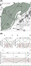Figure 1. (A) Formation extent and play extent of the Marcellus Shale according to the Energy Information Administration (Popova, 2017). (B) Three cross sections—AA′, BB′, and CC′—are constructed without vertical exaggeration from the Marcellus structure and isopach maps in Popova (2017). The limits of gas windows correlate with the subsea depths of 3000 to 6500 ft. NY = New York; OH = Ohio; PA = Pennsylvania; WV = West Virginia.

The EIA outlines 58,000 mi², depicted with the thick dashed line in Figure 1A to delineate the Marcellus play extent, where drilling should be profitable to the operators. To show depth and thickness variations in the Marcellus Shale, we have constructed three cross sections—AA^′, BB^′, and CC^′—based on the structure and isopach maps of the Marcellus from Popova (2017) (see Figure 1B). Based on the absolute thickness and the absolute depth of the Marcellus, we can roughly locate two sweet spots, one in northeastern Pennsylvania and the other at the border between northwestern Virginia and southwestern Pennsylvania. The maps of vitrinite reflectance (R_o) and hydrogen index (HI) from Dolson (2016) also confirm that these two sweet spots are thermally mature for producing dry gas and natural gas liquids, with the R_o values of 1.5% to 2.5% and HI values of 4 to 52.

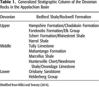
To assess technically recoverable resources in the Marcellus, USGS (Higley et al., 2019) defined six geology-based assessment units (AUs) shown in Figure 2. According to USGS, the potential extent of the Marcellus Shale resources is based on the minimum depth of 1000 ft, minimum thickness of 25 ft, and minimum R_o of 0.5%. The total area of the six AUs is almost identical to the area of the Marcellus Shale by EIA in Figure 1A. The best AUs are denoted by the so-called interior affixes, and their total area is much smaller than that of the EIA’s play extent in Figure 1A. Also note that the two sweet spots identified in Figure 1 are, respectively, inside of the northern interior AU and the southern + southwestern interior AUs.

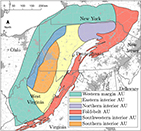Figure 2. The six assessment units (AUs) of the Marcellus Shale according to the US Geological Survey, as described in and modified from Higley et al. (2019).

DESIGN OF WELL COHORTS

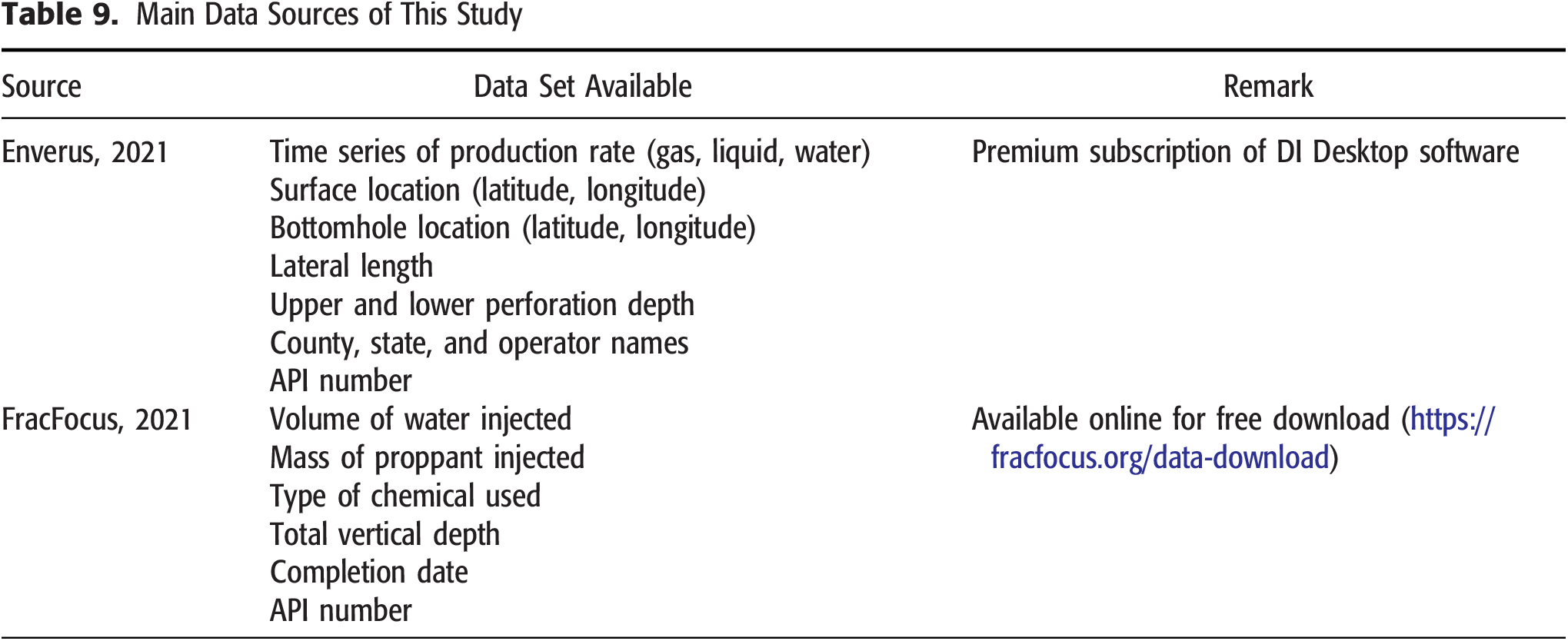
In this paper, we set out to construct several AUs similar to those of USGS (Higley et al., 2019). We base our units solely on well quality, captured as well cohorts. To account for the variations of reservoir quality (geology) in the Marcellus, but also for the changes in completion technologies over time, we make these well cohorts spatiotemporal. For every well in each cohort, the goal is to have similar gas production histories so that each well sample is statistically uniform. The main data sources for this study are obtained from Enverus (2021) and FracFocus (2021), and detailed in the Appendix, Table 9.

First, we divide the Marcellus play extent in space into four reservoir quality areas: the northeast core, southwest core, Marcellus noncore, and Marcellus outer. The two core areas are sweet spots, defined as the envelopes of wells with normalized cumulative production of at least 80 MSCF (see Figure 3). To make a fair comparison between the old and young wells, we divide their cumulative production by the number of elapsed months on production. The shape of the northeast core area follows nicely the USGS northern interior AU in Figure 2, whereas the southwest core area is located in the southern + southwestern interior AUs. These comparisons demonstrate that our core areas also capture the essential geology of the Marcellus, as in Higley et al. (2019). The Marcellus noncore area encompasses the mid-tier wells and is defined as the difference between the effective area and the two core areas. The Marcellus outer area is further defined as the difference between the EIA play boundary and the effective area. It contains subpar wells with normalized cumulative production of less than 20 MSCF.

Figure 3. Scatter map of normalized cumulative production from 12,406 horizontal gas wells in the Marcellus Shale (data adapted from Enverus, 2021) and the outlines of the core areas and the effective area. EIA = Energy Information Administration.

Second, we subdivide the well cohorts in the Marcellus into four completion date intervals: 2009–2012, 2013–2014, 2015–2016, and 2017–2020. This temporal division is based on Figure 4, which shows 10 yr of advancements in well completion technologies in the Marcellus Shale play. From Enverus, we obtain the lateral length data (feet) for 12,401 wells, plotted as gray dots in Figure 4A (Enverus, 2021). Using GEV statistics, we obtain the annual (upper bound), mean (expected value), and (lower bound). From FracFocus, we obtain only 9926 data points for fracturing water volume (gallons) and mass of proppant (pounds) (FracFocus, 2021). We further divide the water volumes and proppant masses for each well in FracFocus by their corresponding lateral lengths from Enverus and obtain the fracturing water intensity (gallons per foot) and proppant intensity (pounds per foot) in the Marcellus (see Figure 4B, C). Since the number of fracture stages for each well is not available, we approximate it by dividing the lateral lengths from Figure 4A with the hydraulic fracture spacing reported from the literature (Gerdom et al., 2013; Eclipse Resources, 2017; Walzel, 2019). In Figure 4D, along with the calculated number of fracture stages, we also show the true values from the literature. From the four time series in Figure 4, we observe a massive completion technology advancement in the Marcellus. Over a decade, the operators almost doubled the lateral lengths and quintupled the number of fracture stages. The increases in fracturing water intensity and proppant intensity may also indicate that more fractures per unit area have been created; hence, reservoir exposure and drainage radius per well have increased.

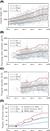Figure 4. Advancement in completion technologies in the Marcellus Shale from 2010 to 2020: (A) lateral length, (B) fracturing water intensity, (C) proppant intensity, and (D) number of stages. P₁₀ = upper bound; P₉₀ = lower bound.

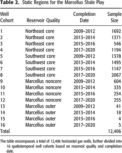
In summary, we divide the Marcellus Shale play into 16 spatiotemporal well cohorts in total (see Figure 5). Table 2 details the sample size numbers included in the cohorts. It is obvious that over the last decade, operators have drilled only in the sweet spots in the two small core areas. Only 12% of the total horizontal wells have been drilled in the Marcellus noncore, and

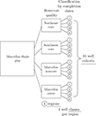Figure 5. The Marcellus Shale well classification used in this paper. All 12,406 horizontal wells in the Marcellus are grouped into 16 spatiotemporal well cohorts based on reservoir qualities and completion dates.

GEV STATISTICS AND HISTORICAL WELL PROTOTYPES

After dividing the Marcellus into 16 spatiotemporal well cohorts, we construct historical well prototypes for each cohort using the GEV statistics. The GEV distributions are used to model numerous extreme events in nature, such as extreme rainfall over a long period, floods, earthquakes, appearance of large pores or fractures in a rock mass, or production of hydrocarbons from fractured shales (Patzek et al., 2019). In statistics, according to the extremal types theorem, the only stable distribution to model such extreme events is GEV distribution, which is able to capture the maxima of long (finite) sequences of random variables. Because measurable gas production in a shale well requires volumetric fracturing of reservoir rock or complex fractures, each production record is an extreme event (Patzek, 2019; Patzek et al., 2019). Therefore, the distributions of annual gas production from the hydrofractured horizontal wells in the Marcellus are accurately fit with GEV distributions.

The previous research by Patzek et al. (2019) and Saputra et al. (2019) shows the superiority of GEV distribution in matching annual gas and oil production in the Barnett and Bakken Shales, compared with the widely used lognormal distribution. The GEV distribution is a generalization of the three extreme value distributions (Fréchet, 1927; Weibull et al., 1951; Gumbel, 1954), each depending on three parameters. In contrast, a normal or lognormal distribution only has two parameters, and . In a symmetrical distribution, is equal to the mean and is the standard deviation. A nonsymmetrical distribution such as GEV may also depend on a third parameter. In a GEV distribution the location parameter is , the scale parameter is , and the shape parameter is . The value of determines which of the three extreme distributions results—Fréchet (), Weibull (), or Gumbel (). In most shale production cases, Fréchet is a better fit because we find that the shape factor, , of annual oil or gas production distributions in several major shale plays in the United States is positive and between 0.1 and 0.2.

The probability density function (PDF) for the GEV distribution is defined as

The GEV cumulative distribution function (CDF) is integration of the PDF:

and the expected value or mean of the GEV distribution is as follows:

Note that a good fit of data with a GEV distribution usually has ξ ξ ≥ 1/2 (see Patzek et al., 2019; Saputra et al., 2019).

Figure 6 demonstrates how we obtain a historical well prototype for each of the 16 Marcellus well cohorts in Table 2. For simplicity, this example focuses on cohort-7, which is the southwest core (2015–2016), with 1147 wells. First, we construct subcohort-7-j, which contains all of the wells in cohort-7 with at least j years on production. For example, there are 1145 wells in the subcohort-7-1 because the other 2 wells in cohort-7 are in the early phases of production, with less than 1 × 12 months on production. Similarly, the subcohort-7-5 has only 450 wells because the other 697 wells in cohort-7 are less than 5 yr old. No subcohort-7-6 is found because cohort-7 only contains wells that were completed in 2015 to 2016.

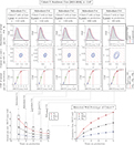Figure 6. Illustration of the approach to obtain historical well prototype for each well cohort. As an example, we pick cohort-7, which samples all of the horizontal gas wells in the southwest core area of the Marcellus Shale, completed between 2015 and 2016. We split cohort-7 into the subcohorts 7-j that contain all of the wells with at least j years on production. In this case, yr. For each subcohort, we fit a generalized extreme value (GEV) distribution and obtain the (upper bound), P₅₀ (mean), and (lower bound) of the annual gas rate (billion standard cubic feet [BSCF]/yr/well). We then connect the , P₅₀, and points from the five subcohorts, and use cumulative production as the stable historical well prototype for cohort-7. = location parameter of GEV PDF; = scale parameter of GEV PDF; CDF = cumulative distribution function; CI = confidence interval; PDF = probability density function.

Second, for each subcohort, we plot the histogram of annual gas rates (BSCF/yr). We then fit a GEV distribution to this histogram, using the GEV PDF in equation 1 with three fitting parameters: , , and . We also display the lognormal distribution fit to show that GEV is better fit to the widely used lognormal distribution in matching annual gas production in shales. The second row in Figure 6 shows the contour plots of and with a corresponding 95% confidence interval. The fewer wells we have in a sample, the wider the uncertainty contour. Because of the fit uncertainty, we discard the subcohorts with fewer than 40 wells. The third row in Figure 6 shows the CDF that can be calculated using equation 2. From the CDF, we can quickly project the (upper bound, or 90th percentile), (median), and (lower bound, or 10th percentile). Using equation 3, we can calculate the mean of each subcohort. Notice that the calculated mean is always higher than the median if we have a positive skewness in the distribution (the heavy tail is on the right-hand side).

Third, we plot the means, , and of the annual gas rate (BSCF/yr/well) of each subcohort versus years on production and calculate the cumulative production (see Figure 6). At this point, we have a complete historical well prototype for cohort-7. We repeat these steps for the other 15 well cohorts in the Marcellus. Each well prototype is constructed solely from the historical production data of existing wells, and it is limited to 5 yr for the cohort-7 wells. In the next step, we use a physical scaling approach to extend the well prototypes for up to two or three more decades. (See SOM-1, supplementary material available as AAPG Datashare 173 at www.aapg.org/datashare, for the individual plots of GEV PDF, GEV contour, and GEV CDF for all 16 cohorts of the Marcellus.) Our approach to obtaining well prototypes from the expected values of GEV distributions is highly predictive. In Figure 7, we demonstrate a cross-validation that GEV means are remarkably stable, even if we omit 50% of the data.

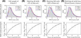Figure 7. To demonstrate the predictive power of our approach, we present a sensitivity analysis (cross-validation) for cohort-7. The four sensitivity cases are (A) base case with 100% data, (B) omitting 5% of the data set at random, (C) omitting 50% of the data set at random, and (D) omitting a cluster of wells. For comparison, we plot the distribution of annual gas rate during the first year on production (prod.), fitted with the lognormal (Logn.) and generalized extreme value (GEV) distributions and the corresponding well prototypes for each sensitivity case. We can see that the GEV approach is remarkably stable and consistent in constructing mean well prototypes, even when 50% of all of the wells are omitted. Cum. = cumulative; BSCF = billion standard cubic feet; PDF = probability density function.

PHYSICAL SCALING AND EXTENDED WELL PROTOTYPES

In addition to the robust GEV statistics, we incorporate physical scaling to extend the historical GEV mean well prototypes for two or three more decades (Patzek et al., 2013, 2014, 2017, 2019; Eftekhari et al., 2018, 2020; Saputra et al., 2020). We adopt this physics-based method instead of the purely empirical industry standard hyperbolic decline curve analysis method (Arps et al., 1945), which tends to overestimate future production (Olson et al., 2019; Haider et al., 2020; Saputra et al., 2020).

The physical-scaling method we use here was originally developed by Patzek et al. (2013, 2014) as a model of nonlinear diffusion of gas pseudo-pressure during gas production from the hydraulically fractured horizontal wells in the Barnett Shale (see Figure 8). They have established that gas production from ≥8000 wells in the Barnett follows a monotonic master curve, along which cumulative gas production grows initially as a straight line versus the square root of time on production (transient period). Later, after 5 to 10 yr, this cumulative production bends down due to an exponential decrease in production rate in pseudo-steady-state flow. This master curve was obtained by solving numerically a nonlinear pseudo-pressure diffusion equation between two consecutive hydraulic fracturing stages. Later, the research by Patzek et al. (2017) and Saputra et al. (2020) produced an exact analytical solution of the physical scaling method for the horizontal black-oil wells in the Eagle Ford and Bakken Shales. We demonstrated that the physical-scaling method is significantly faster than full-scale numerical reservoir simulation, yet it has predictive power that is similar to numerical simulation and other more complex analytical solutions (Saputra and Albinali, 2018).

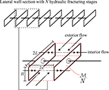Figure 8. Simple physics-based model of oil and gas production in shales. H is the shale formation thickness, 2d is the effective distance between two consecutive hydraulic fractures, and 2L is the tip-to-tip length of the hydraulic fractures. The arrows show the linear flows occurring during the production: from inside the stimulated reservoir volume (SRV) toward the hydraulic fracturing stages (interior flow), and from the outside the SRV toward the lateral section (exterior flow). is the producible hydrocarbon mass per one of the N hydraulic fracture stages per lateral.

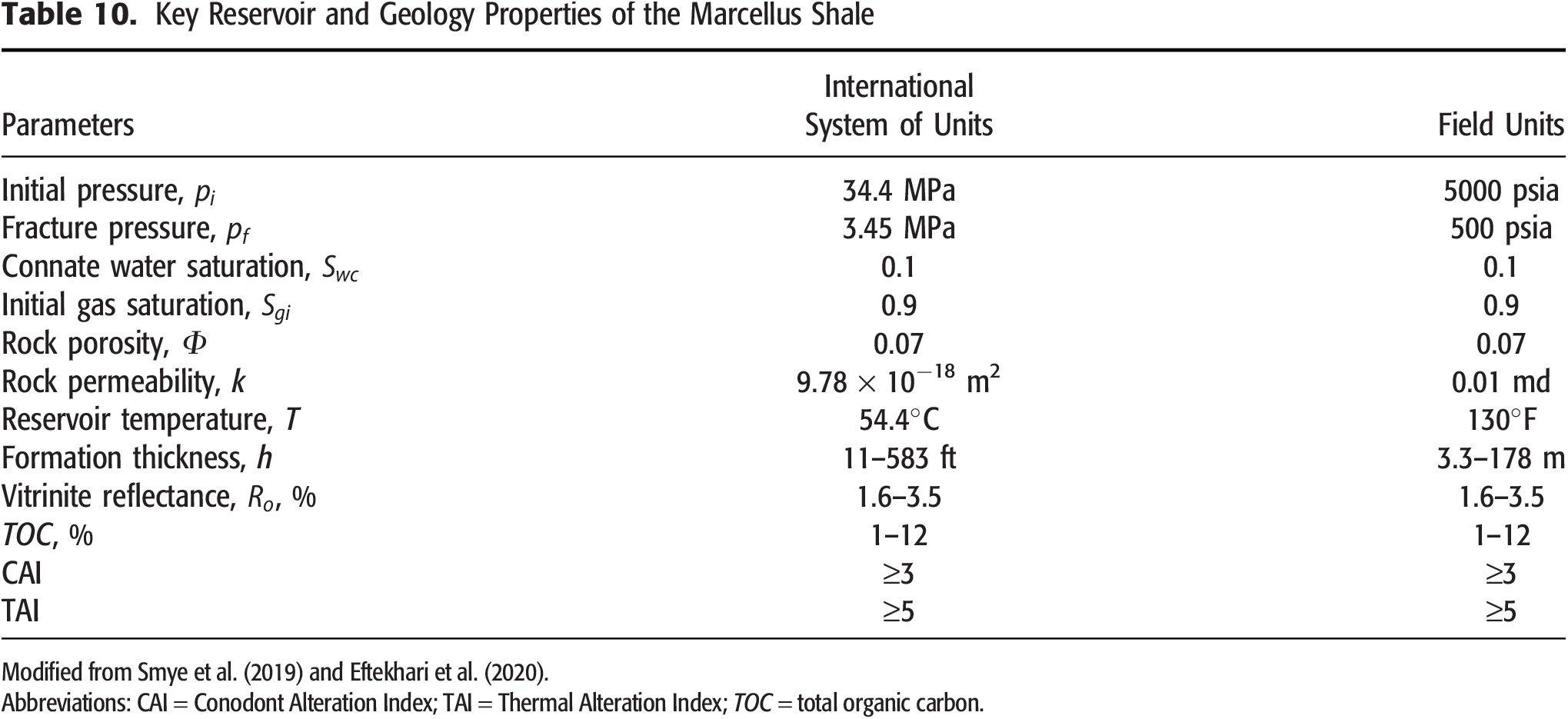
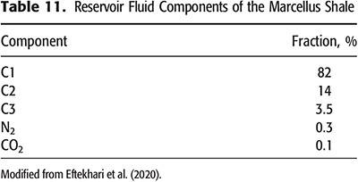
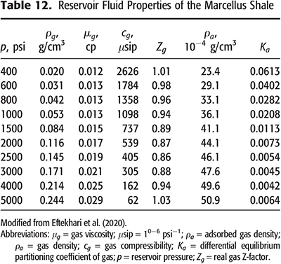
To account for late-time pressure diffusion and gas production, exterior flow from outside the stimulated reservoir volume (SRV) was added to the master curve. This flow appears as an additional square-root-of-time flow scaled by the ratio of hydrofracture spacing to fracture length (Eftekhari et al., 2018). For a shallow and cool gas shale such as the Marcellus, gas adsorption in the matrix is important. Therefore, Eftekhari et al. (2020) modified the pressure diffusion equation to account for additional flow from adsorbed gas. Appendix Tables 10–12 show the key reservoir properties, gas composition, fluid properties, and adsorption parameters used by Eftekhari et al. (2020) to construct the master curve for the Marcellus Shale.

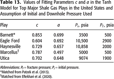
The master curves published in Patzek et al. (2013, 2014) and Eftekhari et al. (2020) were generated from numerical simulations and given as long tables of the recovery factor, RF, versus dimensionless time, , because there is as yet no exact solution for physical scaling in gas wells due to a high nonlinearity of gas properties with pressure. To make this method more engineer friendly, we propose an approximation model that fits satisfactorily each numerical recovery factor in several top shale gas producers in the United States:

where is the dimensionless time and c and a are the fitting parameters listed in the Appendix, Table 13. These parameters depend on gas and adsorption properties and drawdown pressures unique to each shale. Equation 4 was originally published as a three-parameter equation in equation B.1 in Saputra et al. (2021b). In the present paper, we successfully simplified it into a two-parameter equation by discovering that the product of the two fitting parameters a and b is exactly . Consequently, if , is raised to the power of , following the universal emergence of the square root of the time decline rate (Marder et al., 2018, 2021). Figure 9 plots each of the numerical master curves fitted with equation 4.

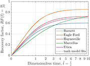Figure 9. Physical scaling for top shale gas producers in the United States. The colored solid lines were obtained from numerical simulation results. The dashed lines are the best fits using equation 4. is the producible hydrocarbon mass per lateral and is the cumulative mass of hydrocarbons produced at the time on production t rendered dimensionless by the division through the pressure interference time .

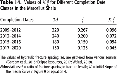
Equation 4 assumes that production only takes place from the interior of the SRV, illustrated as perpendicular bilinear flow toward the hydraulic fractures in Figure 8. If we assume that produced gas originates also in the exterior of the SRV, then the master curve is amended as follows:

where d is the half-distance between two hydraulic fractures, L is the half-length of hydraulic fractures (see Figure 8), and is the initial slope of the master curve in Figure 9 or equation 4 with respect to , which is approximately 0.36 for the Marcellus. Because of the advancement of completion technologies in the Marcellus Shale, the values of change over time as listed in the Appendix, Table 14.

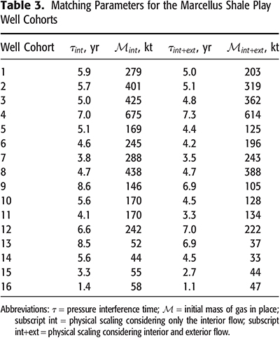
Figure 10 demonstrates the use of the physical scaling method to extend the historical well prototypes over up to two or three more decades. The thick black lines are the cumulative GEV means of annual gas rate (historical well prototypes) that were described in the previous section. After unit conversion from billion standard cubic feet to kilotons, we then match each of the historical well prototypes to the master curves in equation 4 or equation 5. The matching process is by scaling the x-axis, years on production, by the pressure interference time, , and by scaling the y-axis, cumulative mass produced, by the mass of initial gas in place, . Table 3 lists the two matching parameters, and , for all 16 well cohorts.

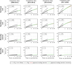Figure 10. Extended well prototypes for the 16 well cohorts in the Marcellus Shale. Each row highlights different reservoir qualities and each column signifies different completion dates. Every point of the black line traces the expected values (means) of the generalized extreme value distributions of all of the active horizontal gas wells in each well cohort. The dashed lines labeled and denote wells whose cumulative production is exceeded by 10% and 90% of wells in each region (upper bound and lower bound, respectively). The physics-based scaling curves that match each average well with and without exterior flow during late time production are denoted by the green (with) and red (without) lines.

The physical scaling matches are shown in Figure 10 as the red and green lines. We determine EUR from each well cohort by looking at the endpoint of each physical scaling projection. We infer that the northeast core is the best region of the Marcellus, with EURs of up to 15 BSCF/well, followed by the southwest core with EURs of up to 11.5 BSCF/well. From a geological perspective (Dolson, 2016; Higley et al., 2019), the northeast core is more mature (dry gas) and has a thicker shale layer than the southwest core. Thus, its productivity is higher. The Marcellus noncore is less productive, with EUR lower by two- to threefold. The worst producing region is the Marcellus outer, which produces merely 1–2 BSCF/well, so that nobody has drilled in this area up until the present. From Figure 10, we conclude that the advancement of completion technologies helps to boost production almost twofold for both the northeast and southwest cores (comparing the oldest to newest cohorts). However, for the Marcellus noncore and Marcellus outer, where reservoir quality is poor, these technologies most likely do not help much.

PROBABILITY OF WELL SURVIVAL

Well prototypes obtained from GEV statistics and physical scaling are highly idealized, with oil or gas production that lasts for decades. In reality, production from shale wells may not last that long in most cases. The reduction in reservoir pressure, increase in water cut, closure and deterioration of hydraulic fractures, and reduction of effective rock permeability decrease well production rates in shales.

When well production falls below an economic limit set by an operator, this operator then shuts in the well. Therefore, it is important to determine when particular wells may become inactive for a variety of reasons. To do so, we first calculate the probability of well survival in each subregion of the Marcellus:

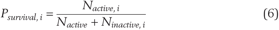
where N_active,i and N_inactive,i are the numbers of active and inactive wells in year i. If we plot P_survival for a well cohort in a region of a play versus year on production, and fit a parabolic curve, then the intercept of that curve at P_survival = 0 defines the maximum time of well survival, t_max (months).

Figure 11 displays the probabilities of well survival of the northeast core and southwest core wells (see SOM-2, supplementary material available as AAPG Datashare 173 at www.aapg.org/datashare, for all of the Marcellus regions). Each color represents a different year of completion. In both plots, the dotted line is the average of endpoint probabilities of survival of all of the well cohorts. The dashed line is a parabolic fit of the oldest well cohort that intercepts the maximum time of well survival, t_max, at which P_survival = 0. We can see that wells in the northeast core survive longer than the wells in the southwest core. This may be due to different maturity levels of the reservoir rock. The southwest core is less mature, and we expect that there may be condensate banking near the wellbore that prohibits the wells from surviving for a longer time.

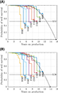Figure 11. Probability of survival for (A) the northeast core area and (B) the southwest core area. The colored stairstep lines represent well survival probabilities for different completion years. For instance, in the northeast core area, only 75% of wells completed in 2009 survived after 11 yr. The newer wells survive less longer, so that the average survival probability is only 52%. Finally, from a parabolic extrapolation, we obtain the maximum time of well survival of 14 yr.

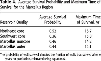
Table 4 summarizes the average probability of well survival and maximum time of survival for each subregion of the Marcellus. We use these values to stop production of each well prototype shown in Figure 10.

BASE FORECAST

To confirm that we have obtained robust and stable well prototypes, we replace the production rate from each existing well with its corresponding well prototype, time shifted to the date of first production from the actual well, and sum up. The summation should match closely the historical gas rate. Figure 12 shows the result of this procedure for 12,406 existing wells in the Marcellus. The red and green curves are the physical scaling forecasts with and without exterior flow that match the black historical production curve. Both physical scaling projections forecast the play’s EUR of approximately 85 TSCF by 2030.

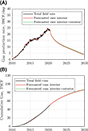Figure 12. (A) Actual and forecasted total field rate and (B) cumulative (cum) gas production in the Marcellus Shale. This forecast is a do-nothing scenario, assuming that there are no future drilling programs and the production comes from the existing 12,406 horizontal wells in the Marcellus. BSCF = billion standard cubic feet; TSCF = trillion standard cubic feet.

We call this projection a base or do-nothing scenario of shale play development, in which there is no further drilling of new wells. This is the case for the already overdrilled, mature Barnett (Patzek et al., 2019) and Fayetteville plays, or if a global crisis hits the oil industry so hard that investment dries up and operators stop drilling new wells. In the Marcellus, if the operators stopped drilling today, then the total field gas rate would drop by half in just 3 yr. This is the true nature of shale play development, in which massive drilling must continue to maintain stable production. In the next three sections, we discuss in detail how we predict future infill drilling in the Marcellus.

PROBABILITY OF SUCCESS

Before we calculate how many wells are available for future drilling programs, we should calculate the probability of success for each subregion in a shale play. To do so, we cover each subregion with rectangular grid cells, in which each cell is 1 × 1 mi. From Enverus (2021), we determine a dry well if gas production is zero and the well status is permanently shut in, plugged, or abandoned. If a cell contains at least one dry well, we label it a dry cell; otherwise, it is a nondry cell. We later count the number of dry cells as N_dry and the number of nondry cells as N_nondry. The probability of successfully finding the nondry (productive) wells can be calculated as follows:

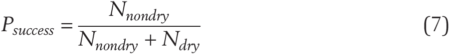
Figure 13 shows the distribution of tested cells in the northeast and southwest cores (see SOM-2, supplementary material available as AAPG Datashare 173 at www.aapg.org/datashare, for all of the Marcellus regions). The orange cells are locations where productive wells exist and the black cells are locations for dry hole wells.

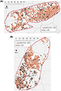Figure 13. Map of tested cells in (A) the northeast core and (B) the southwest core of the Marcellus Shale. The probability of success for each region is calculated as a fraction between the number of productive cells (orange) and the total number of tested cells (orange + black).

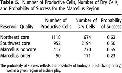
The number of productive and dry cells and the probability of success for each Marcellus subregion are summarized in Table 5. The highest probability of success exists in the northeast core of the Marcellus, whereas it is lowest in the Marcellus outer, as expected. However, these values are relatively low compared to a more mature shale play (e.g., Haynesville) (Saputra et al., 2021b), in which the probability of success is more than 90% (9 out of 10 wells drilled in Haynesville are expected to be productive). An immature shale tends to have a water saturation that is higher than those of oil or gas (Patzek et al., 2019; Saputra et al., 2019). If the effective permeability to water is higher than those to hydrocarbons, then the wells are expected to flow little or no oil or gas, leading to dry wells.

INFILL POTENTIAL

In this section, we calculate the number of potential infill wells to be drilled. This calculation is similar to the previous one. First, we cover each subregion of the Marcellus with the 1-mi² grid cells. Due to regulatory restrictions, it is impractical to drill and produce inside-city boundaries. Therefore, we exclude every grid cell that intersects urban areas, shown as the dark gray areas in Figure 3.

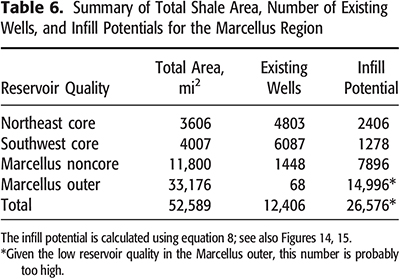
Second, we use equation 8 to calculate the number of potential infill wells in each of the subregions of the Marcellus:

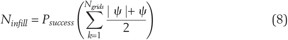
where N_grids is the total number of 1-mi² grids in each subarea, is the difference between the maximum allowable number of wells per square mile to avoid fracturing hits and the number of existing wells per grid cell, and P_success is the probability of success that we calculated in the previous section.

Figures 14 and 15 help demonstrate the calculation of potential infill wells in the Marcellus by showing the lateral directions, well density, and infill potential maps of the northeast and southwest cores of the Marcellus (see SOM-2, supplementary material available as AAPG Datashare 173 at www.aapg.org/datashare, for all subregions of the Marcellus). From Figures 14A and 15A, we observe how operators adapt to the direction of minimum horizontal stress in the Appalachian Basin. To generate stable transverse vertical hydraulic fractures, the operators should drill wells at ∼S20°E in the northeast core and ∼S45°E in the southwest core.

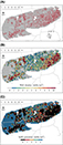Figure 14. (A) Lateral directions for 4811 existing horizontal wells, (B) well density, and (C) infill potential maps of the northeast core area in the Marcellus Shale. For this region, the typical well orientation is S20°E, which reflects the direction of minimum horizontal stress. Well density is the total number of horizontal wells that intersect each of the 1-mi² grid cells. The infill potential is calculated using equation 8.

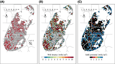Figure 15. (A) Lateral directions for 6120 existing horizontal wells, (B) well density, and (C) infill potential maps of the southwest core area in the Marcellus. The typical well orientation is approximately S45°E for this region. As in Figure 14, the infill potential map is calculated using equation 8.

For each grid cell, we count how many wells intersect this cell in the subsurface. The outcome is the subsurface well density maps shown in Figures 14B and 15B. The different colors show how many wells already exist per square mile. Following Saputra et al. (2019, 2021b), we assume that the maximum allowable number of wells to be drilled is 4 wells/mi² for a typical fracture length of 1200 ft. Based on equation 8, we calculate by subtracting each well density map from the assumed maximum allowable number of wells. Figures 14C and 15C show the results as . Notice that a negative converts to zero in both maps, suggesting overdrilling in each black grid cell.

Finally, we sum the potential infill wells for all grid cells and multiply the result by the probability of success. The results are tabulated in Table 6.

INFILL FORECAST

Based on the infill potentials in Table 6 and historical drilling rates in Figure 16A, we schedule the future drilling programs shown in Figure 16B. We have obtained the number of active rigs (rig count) in the Appalachian Basin from EIA, and the number of horizontal wells completed per month (drilling rates) from Enverus (2021). It is interesting to see that after 2020, the monthly rig counts match perfectly the drilling rates. We also highlight three levels of drilling rates: 130 wells/month in 2011 to 2015, with gas prices above $10/MSCF; 80 wells/month in 2017 to 2019, with gas prices recovering after the 2008–2009 financial crisis to >$3/MSCF; and 50 wells/month during the oil crisis of 2016, followed by the global coronavirus disease 2019 pandemic of 2020 to 2021.

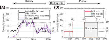Figure 16. (A) Historical rig count and drilling rate of horizontal gas wells in the Marcellus Shale. (B) Scheduled infill drilling rate in the Marcellus Shale assuming three variable drilling rates: 50, 80, and 130 wells/month. The roman numerals denote the end of infill potentials for the (i) northeast core, (ii) southwest core, (iii) Marcellus noncore, and (iv) Marcellus outer. Note that the infill outer scenario is not possible based on current gas prices (see the Economic Analysis section). EIA = Energy Information Administration.

Based on Table 2, we observed that operators mostly drill in the core areas. Therefore, we continue this trend and schedule to drill first the 2406 and 1278 potential wells in the northeast and southwest cores, respectively, using the historically low drilling rate of 50 wells/month. With this infill drilling program in place, in 2027, it is expected that no well locations will be left in the core areas. Thus, operators may be forced to move to the less productive Marcellus noncore and drill all of the potential 7896 wells at a higher drilling rate of 80 wells/month. Here, we assume that the industry will recover by 2027. By 2035, there should be no new locations left for infill drilling in the core and noncore areas of the Marcellus. Thus, operators may be able to drill only the least productive Marcellus outer area at the most optimistic drilling rate of 130 wells/month. In the next section, we demonstrate that drilling ∼15,000 wells in the unproductive outer area is economically unfeasible, except at high gas prices.

Using an approach similar to that in the previous section, we replace the future wells scheduled in the drilling programs in Figure 16B with their corresponding time shifted well prototypes and sum up the resulting rates to obtain the total field rate. In Figure 17A, we show the total field rate as the increments from the base or do-nothing case in Figure 12. We gradually infill both core areas and then the noncore area; finally, we infill the Marcellus outer area. By drilling in the core areas, we can maintain a production plateau of approximately 25 BSCF/day for the next 5 yr. Even if we increase the drilling rate from 50 to 80 wells/month, the infill in the noncore area does not prevent production from declining. The most optimistic and highly unlikely infill scenario of 130 wells/month in the outer area still cannot save the Marcellus from its terminal decline.

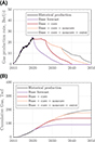Figure 17. The predicted total field rate (A) and cumulative gas (B) for the Marcellus Shale based on the infill scenario in Figure 16. Note that the purple lines are the do-nothing production forecasts from the 12,406 existing wells introduced in Figure 12. The red lines correspond to drilling 3684 best potential wells in the core area. The orange lines depict drilling 7896 less-productive wells in the noncore area. Finally, the dark gray lines are the least likely scenario when operators are desperate enough to drill ∼15,000 least-productive wells in the outer area. BSCF = billion standard cubic feet; TSCF = trillion standard cubic feet.

Finally, we integrate the total field rates in Figure 17A to predict the ultimate recoveries from the Marcellus (see Figure 17B). The 12,406 existing wells in the Marcellus are predicted to ultimately produce 85 TSCF of gas by 2040. By adding the 3684 potential wells in the core areas, the cumulative production is poised to increase to ∼150 TSCF by 2040. The additional 7896 wells in the noncore area may increase the ultimate production to only ∼180 TSCF by 2050. Lastly, the staggering number of 15,000 wells in the outer area may yield only an additional ∼20 TSCF, an endeavor that is economically unfeasible, as we discuss in the next section.

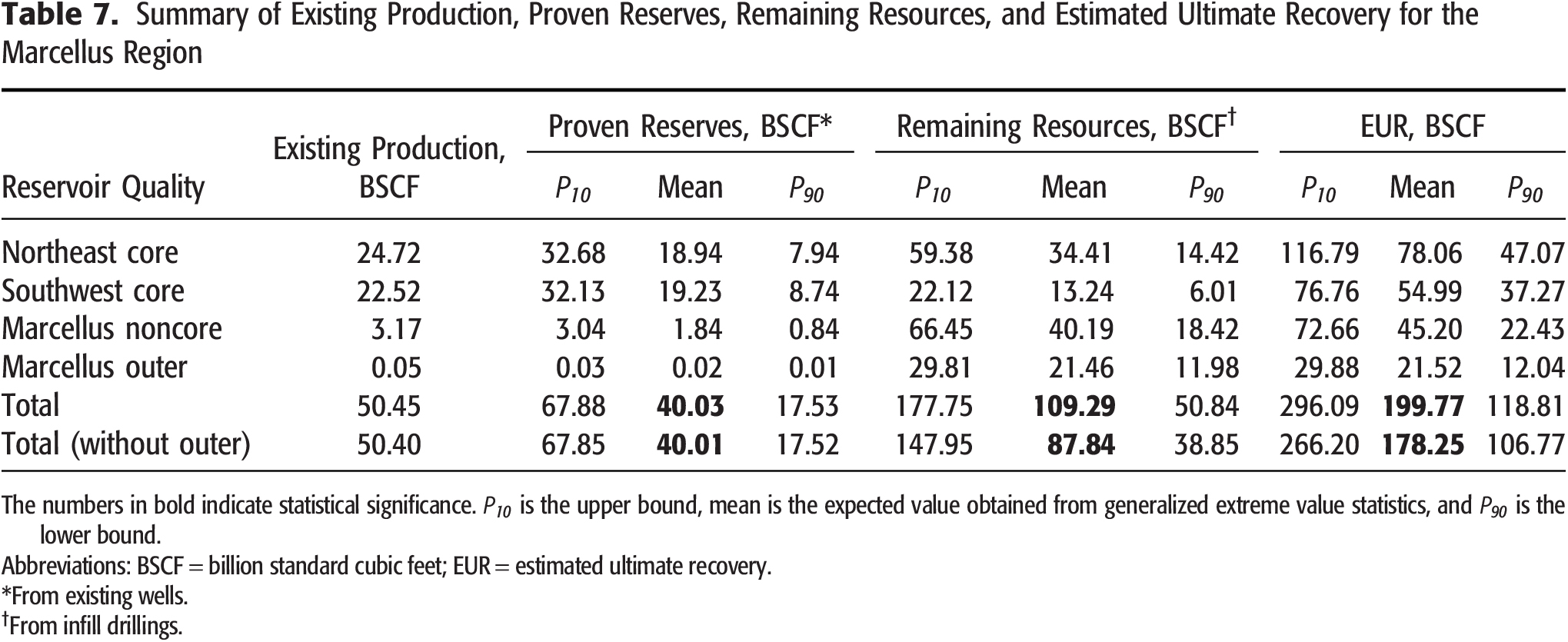
In Table 7, we summarize the existing production, proven reserves, remaining resources, and EUR from four different reservoir qualities of the Marcellus. Besides the expected values (mean), we also present the upper bounds () and the lower bounds () of each estimated reserve–resource based on GEV statistics. We also compare the results of this study with other published results (Ikonnikova et al., 2018; Higley et al., 2019; Energy Information Administration, 2020a) (see Table 8). Our estimate of the remaining resources at 88 to 109 TSCF is highly similar to what USGS predicted in 2019, at 96.5 TSCF. Next, we translate the value of the remaining resources into EUR or TRR by adding existing production and proven reserves. Our predicted TRR value at 178 to 200 TSCF is much lower than what EIA and BEG predicted at 310.6 and 560 TSCF, respectively.

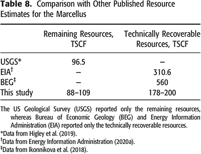
To clarify, our analysis was completed solely for the Marcellus. The USGS prediction is also based on the Marcellus layer at a similar target depth, and this is probably why our estimates are so similar. There may be additional potential production coming from the adjacent formations, such as the Upper Devonian Marcellus. (However, as of January 2021, there were only 399 wells producing from the Upper Devonian interval, and their production was negligible compared with the ≥15,000 wells drilled in the Marcellus.) Perhaps EIA and BEG also considered these additional layers, and therefore their estimates were two to three times higher than ours. The lower ultimate resource estimates proposed in this paper are supportable, we think, from the high statistical confidence we have in well productivity obtained with the approach taken.

ECONOMIC ANALYSIS

In this section, we quantify which of the Marcellus wells are profitable, given the present state of drilling and completion technologies and gas prices. To compare the profitability of each drilling project in each subregion of the Marcellus, we adopt the concept of net present value (NPV) from Kaiser (2012) and Saputra et al. (2021a, b). The concept of NPV is based on the assertion that every dollar invested today ought to bring profit over the next 8 yr or longer. The accruing increase in value of the initial investment is measured by the discount rate (DIS). If the net cash flow (NCF) in year i (NCF_i; i = 0,1,2,...,t_max) is NCF_i, then the total NPV is

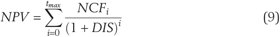
where t_max is the lifetime of the project. In this case, it is the maximum time on production that we have calculated from the probability of well survival in a given area of the Marcellus. A profitable project should yield a positive NPV, whereas a negative NPV means a money loss. When NPV, we call it breakeven, which occurs at a certain gas price. Our goal is to calculate the NPV of each drilling project and determine the gas price at which the breakeven of that project happens. The lower the breakeven price, the better the project.

We calculate NCF for each year on production, NCF_i, in SOM-3 (supplementary material available as AAPG Datashare 173 at www.aapg.org/datashare). Equation 10 states that during each year i, the NCF is the gross revenue (GR), minus the capital expenditure (CAPEX), minus the operating expenditure (OPEX), minus the royalty (ROY), and minus the taxes (TAX):

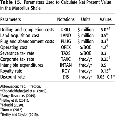
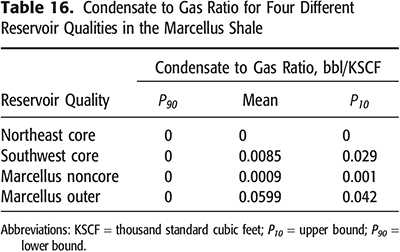
Table 15 in the Appendix lists the economic parameters used to calculate the NPVs of different development scenarios in the Marcellus Shale. We have obtained these parameters from various sources (Hefley and Seydor, 2011, 2015; Duman, 2012; Khodabakhshnejad et al., 2019; Range Resources, 2019; Tabuchi, 2020). The gross revenue is the summation of annual gas and natural gas liquid (NGL) production multiplied by the gas and NGL prices, respectively. Using GEV statistics, we calculate the expected value of condensate to gas ratio that can be used to estimate the amount of NGL produced (see the Appendix, Table 16). The capital expenditure is the summation of drilling and completion cost (∼$5 million), land acquisition cost (∼$0.5 million), and plug and abandonment cost (∼$0.3 million). The operating expenditure is the total annual gas and NGL production (in barrels of oil equivalent [BOE]) multiplied by the operating cost (∼$4.2/BOE). The royalty is the gross revenue multiplied by the royalty rate (∼15%/yr). The overall tax rate is the most difficult parameter to calculate (see SOM-3, supplementary material available as AAPG Datashare 173 at www.aapg.org/datashare for details). To calculate taxes, we need to assume the severance tax rate (∼$0.3/BOE), corporate tax rate (∼25%/yr), and intangible expenditure (∼50%/yr). Finally, the 10% DIS is chosen because it is widely used in the annual reports of United States oil and gas companies.

In the present study, we use two scenarios of NPV calculations for four reservoir qualities in the Marcellus. We show the results in Figure 18. In the first scenario, we fix the NGL price at $31.5/bbl as of August 2021 (Cocklin, 2021b) while varying the gas price to determine at what gas prices the infill project breaks even. In the second scenario, we fix the gas price at $2.81/thousand SCF (KSCF) as of August 2021 (Cocklin, 2021a) and vary the NGL prices. The detailed NPV calculations at different gas and NGL prices are tabulated in SOM-3 (supplementary material available as AAPG Datashare 173 at www.aapg.org/datashare).

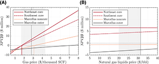Figure 18. Net present values (NPV) at 10% discount rate (NPV10) for four different reservoir qualities in the Marcellus Shale calculated at (A) various gas prices and a constant natural gas liquids (NGL) price at $32/bbl, and (B) various NGL prices and a constant gas price at $2.81/thousand SCF. The thick vertical line and the gray area show the gas or NGL price in August 2021 and range of gas or NGL prices for the previous 6 months.

In Figure 18A, we see that both core areas (northeast and southwest) have similar breakeven points at a gas price less than $1.8/KSCF. The Marcellus noncore is less productive than the core areas, and thus the breakeven point shifts to $3.1/KSCF. As expected, the least productive Marcellus outer has the highest breakeven point at $7/KSCF. For comparison, a comprehensive study by the Journal of Petroleum Technology (2019) shows similar breakeven prices for the Marcellus, ranging from $1 to $8/KSCF.

In Figure 18B, we see the impact of NGL prices on the profitability of each infill project. The northeast core contains only dry gas with no NGL production, so that the NPV remains constant whatever the NGL price. However, the southwest core yields a significant amount of NGL, so that the higher the NGL price, the more profitable the infill project. Lastly, both Marcellus outer noncore and Marcellus outer give negative NPV for all NGL prices shown in the graph, and they are not profitable at current prices.

From this exercise, one can infer that drilling in both the Marcellus northeast and southwest core areas may always yield a positive cash flow, even if gas prices plunge below $2/KSCF. The Marcellus noncore area may be an alternative for infill drilling if gas prices exceed $3/KSCF. Finally, we do not recommend drilling in the Marcellus outer area because it is expected to generate negative cash flows, unless gas prices increase to more than $7/KSCF, which is unlikely in this era of low oil and gas prices.

CONCLUSIONS

We have provided an optimal play-wide assessment of the Marcellus Shale by considering the shale play geology, advancement of well completion technologies, physics of natural gas production from the horizontal hydraulically fractured wells, and economics of drilling projects.

Our GEV statistics approach makes all of the well prototypes robust and in excellent agreement with the physics-based scaling curves. Using these prototypes, we were able to match rather well the historical gas production from the entire Marcellus Shale.

Both core areas in the northeast and the southwest of the Marcellus give the highest EUR and the most profitable wells due to the more mature and thicker Marcellus Formation.

The newer wells yield higher EURs due to (1) longer lateral lengths, (2) larger hydraulic fractures, and (3) more hydraulic fracture stages. However, in areas of poor reservoir quality, these advancements in completion technologies cannot help much.

Ultimately, the 12,406 existing wells in the Marcellus are expected to produce 85 TSCF of natural gas by 2040. By adding another 3864 and 7896 potential wells in the core and noncore areas, the ultimate recovery is poised to increase to 150 and 180 TSCF, respectively.

Operators should not bother with drilling in the outer area of the Marcellus because it may be unprofitable for all of the scenarios we considered. Other attractive shale plays should be drilled that may yield higher cash flows (e.g., Haynesville Formation and Utica Shale).

In our opinion, the hybrid data-driven and physics-based approaches are the future of production forecasting and reserve estimation in all shale plays. These methods deliver the best—in the least squares sense—predictions of possible futures, are free from bias, and avert significant over- or underpredictions of reserves.

REFERENCES CITED

Arps, J. J., 1945, Analysis of decline curves: Transactions of the AIME, v. 160, no. 1, p. 228–247, doi:10.2118/945228-G.
BP, 2020, Statistical review of world energy: London, BP, v. 69, 68 p.
Carter, K. M., J. A. Harper, K. W. Schmid, and J. Kostelnik, 2011, Unconventional natural gas resources in Pennsylvania: The backstory of the modern Marcellus Shale play: Environmental Geoscience, v. 18, no. 4, p. 217–257, doi:10.1306/eg.09281111008.
Cipolla, C. L., R. E. Lewis, S. C. Maxwell, and M. G. Mack, 2011, Appraising unconventional resource plays: Separating reservoir quality from completion effectiveness: International Petroleum Technology Conference, Bangkok, Thailand, November 15–17, 2011, IPTC-14677-MS 27 p., doi:10.2523/IPTC-14677-MS.
Cocklin, J., 2021a, Cabot, Southwestern see natural gas prices impacted by Appalachian pipeline constraints, accessed August 10, 2021, https://www.naturalgasintel.com/cabot-southwestern-see-natural-gas-prices-impacted-by-appalachian-pipeline-constraints.
Cocklin, J., 2021b, Range Resources reports highest ever NGL premium amid booming international demand, accessed August 10, 2021, https://www.naturalgasintel.com/range-resources-reports-highest-ever-ngl-premium-amid-booming-international-demand.
Dolson, J., 2016, Understanding oil and gas shows and seals in the search for hydrocarbons: New York, Springer, 505 p., doi:10.1007/978-3-319-29710-1.
Duman, R. J., 2012, Economic viability of shale gas production in the Marcellus Shale; Indicated by production rates, costs and current natural gas prices, M.S. thesis, Michigan Technological University, Houghton, Michigan, 218 p.
Eclipse Resources, 2017, 2017 analyst day presentation, 77 p., accessed September 7, 2023, https://marcellusdrilling.com/wp-content/uploads/2017/02/Analyst_Day_Presentation_FINAL.pdf.
Eftekhari, B., M. Marder, and T. W. Patzek, 2018, Field data provide estimates of effective permeability, fracture spacing, well drainage area and incremental production in gas shales: Journal of Natural Gas Science and Engineering, v. 56, p. 141–151, doi:10.1016/j.jngse.2018.05.027.
Eftekhari, B., M. Marder, and T. W. Patzek, 2020, Estimation of effective permeability, fracture spacing, drainage area, and incremental production from field data in gas shales with nonnegligible sorption: SPE Reservoir Evaluation & Engineering, v. 23, no. 2, p. 664–683, doi:10.2118/199891-PA.
Energy Information Administration, 2020a, Assumptions to the annual energy outlook 2020: Oil and gas supply module, 81 p., accessed September 7, 2023, https://www.eia.gov/outlooks/aeo/pdf/AEO2020%20Full%20Report.pdf.
Energy Information Administration, 2020b, Natural gas explained: Use of natural gas, accessed November 1, 2020, https://www.eia.gov/energyexplained/natural-gas/use-of-natural-gas.php.
Enverus, 2021, DI Desktop software by Enverus, accessed January 13, 2021, https://www.enverus.com/blog/the-new-drillinginfo-home-page-your-portal-to-the-patch/.
FracFocus, 2021, Data download, accessed January 13, 2021, https://fracfocus.org/data-download/.
Fréchet, M., 1927, Sur la loi de probabilité de l’écart maximum: Annales de la Société Polonaise de Mathematique, v. 6, p. 93–116.
Fulford, D. S., 2016, Unconventional risk and uncertainty: Show me what success looks like: Society of Petroleum Engineers/International Association for Energy Economics Hydrocarbon Economics and Evaluation Symposium, Houston, Texas, May 17–18, 2016, SPE-179996-MS, 43 p., doi:10.2118/179996-MS.
Gerdom, D., J. Caplan, I. Terry Jr., K. Wutherich, E. Wigger, and K. Walker, 2013, Geomechanics key in Marcellus wells: American Oil & Gas Reporter, v. 56, no. 3, p. 84–91.
Gumbel, E. J., 1954, Statistical theory of extreme values and some practical applications: A series of lectures: Washington, DC, National Bureau of Standards Applied Mathematics Series, 60 p.
Haider, S., W. Saputra, and T. Patzek, 2020, The key factors that determine the economically viable, horizontal hydrofractured gas wells in mudrocks: Energies, v. 13, no. 9, 2348, 22 p., doi:10.3390/en13092348.
Harper, J. A., 2008, The Marcellus Shale: An old “new” gas reservoir in Pennsylvania: Pacific Geology, v. 38, no. 1, p. 2–13.
Haskett, W. J., and P. J. Brown, 2005, Evaluation of unconventional resource plays: Society of Petroleum Engineers Annual Technical Conference and Exhibition, Dallas, Texas, October 9–12, 2005, SPE-96879-MS, 11 p., doi:10.2118/96879-MS.
Hefley, B., S. Seydor, M. K. Bencho, I. Chappel, M. Dizard, J. Hallman, J. Herkt, P. J. Jiang, M. Kerec, F. Lampe, , 2011, The economic impact of the value chain of a Marcellus Shale well: Pittsburgh, Pennsylvania, University of Pittsburgh Katz Graduate School of Business, 92 p., doi:10.2139/ssrn.2181675.
Hefley, W. E., and S. M. Seydor, 2015, Direct economic impact of the value chain of a Marcellus Shale gas well, in W. E. Hefley and Y. Wang, eds., Economics of unconventional shale gas development: New York, Springer, p. 15–45, doi:10.1007/978-3-319-11499-6_2.
Higley, D. K., C. E. Enomoto, H. M. Leathers-Miller, G. S. Ellis, T. J. Mercier, C. J. Schenk, M. H. Trippi, , 2019, Assessment of undiscovered gas resources in the Middle Devonian Marcellus Shale of the Appalachian Basin province, 2019, Fact Sheet 2019-3050, 2 p., accessed October 20, 2020, https://pubs.er.usgs.gov/publication/fs20193050.
Hughes, J. D., 2013, A reality check on the shale revolution: Nature, v. 494, no. 7437, p. 307–308, doi:10.1038/494307a.
Ikonnikova, S. A., K. Smye, J. Browning, R. Dommisse, G. Gülen, S. Hamlin, S. Tinker, F. Male, G. McDaid, and E. Vankov, 2018, Update and enhancement of shale gas outlooks, Report No. DOE-BEG-0026962, 60 p., accessed October 20, 2020, https://www.osti.gov/biblio/1479289.
Journal of Petroleum Technology, 2019, Enverus forecasts “significant slowdown” in US gas output, accessed April 20, 2020, https://jpt.spe.org/enverus-forecasts-significant-slowdown-us-gas-output-growth-2020.
Kaiser, M. J., 2012, Haynesville shale play economic analysis: Journal of Petroleum Science Engineering, v. 82–83, p. 75–89, doi:10.1016/j.petrol.2011.12.029.
Khodabakhshnejad, A., A. R. Zeynal, and A. Fontenot, 2019, The sensitivity of well performance to well spacing and configuration—A Marcellus case study: Unconventional Resources Technology Conference, Denver, Colorado, July 22–24, 2019, URTeC-1076, p. 331–344.
Marder, M., B. Eftekhari, and T. W. Patzek, 2018, Solvable model for dynamic mass transport in disordered geophysical media: Physical Review Letters, v. 120, no. 13, 138302, 4 p., doi:10.1103/PhysRevLett.120.138302.
Marder, M., B. Eftekhari, and T. W. Patzek, 2021, Solvable model of gas production decline from hydrofractured networks: Physical Review E, v. 104, no. 6, 065001, 21 p., doi:10.1103/PhysRevE.104.065001.
Milici, R. C., and C. S. Swezey, 2014, Assessment of Appalachian Basin oil and gas resources: Devonian gas shales of the Devonian Shale-Middle and Upper Paleozoic total petroleum system, in L. F. Ruppert and R. T. Ryder, eds., Coal and petroleum resources in the Appalachian Basin: Distribution, geologic framework, and geochemical character: Reston, Virginia, US Geological Survey, 81 p., doi:10.3133/pp1708G.9.
Olson, B., R. Elliott, and C. M. Matthews, 2019, Fracking’s secret problem–Oil wells aren’t producing as much as forecast, accessed April 1, 2020, https://www.wsj.com/articles/frackings-secret-problemoil-wells-arent-producing-as-much-as-forecast-11546450162.
Patzek, T., 2019, Barnett Shale in Texas: Promise and problems: Austin, Texas, Texas Data Repository, 172 p., doi:10.18738/T8/3MLRLO.
Patzek, T. W., F. Male, and M. Marder, 2013, Gas production in the Barnett Shale obeys a simple scaling theory: Proceedings of the National Academy of Sciences of the United States of America, v. 110, no. 49, p. 19731–19736, doi:10.1073/pnas.1313380110.
Patzek, T. W., F. Male, and M. Marder, 2014, A simple model of gas production from hydrofractured horizontal wells in shales: AAPG Bulletin, v. 98, no. 12, p. 2507–2529, doi:10.1306/03241412125.
Patzek, T. W., W. Saputra, and W. Kirati, 2017, A simple physics-based model predicts oil production from thousands of horizontal wells in shales: Society of Petroleum Engineers Annual Technical Conference and Exhibition, San Antonio, Texas, October 9–11, 2017, SPE-187226-MS, 26 p., doi:10.2118/187226-MS.
Patzek, T. W., W. Saputra, W. Kirati, and M. Marder, 2019, Generalized extreme value statistics, physical scaling, and forecasts of gas production in the Barnett Shale: Energy & Fuels, v. 33, no. 12, p. 12154–12169, doi:10.1021/acs.energyfuels.9b01385.
Popova, O., 2017, Marcellus Shale play: Geology review, accessed January 10, 2021, https://www.eia.gov/maps/pdf/MarcellusPlayUpdate_Jan2017.pdf.
Range Resources, 2019, Range announces fourth quarter and year-end 2019 results, accessed July 13, 2019, https://www.globenewswire.com/news-release/2020/02/27/1992332/0/en/Range-Announces-Fourth-Quarter-and-Year-End-2019-Results.html.
Saputra, W., 2021, Physics-guided data-driven production forecasting in shales, Ph.D. thesis, King Abdullah University of Science and Technology, Thuwal, Saudi Arabia, 256 p., doi:10.25781/KAUST-OI7LM.
Saputra, W., and A. A. Albinali, 2018, Validation of the generalized scaling curve method for EUR prediction in fractured shale oil wells, Society of Petroleum Engineers Kingdom of Saudi Arabia Annual Technical Symposium and Exhibition, Dammam, Saudi Arabia, April 23–26, 2018, SPE-192152-MS, 14 p., doi:10.2118/192152-MS.
Saputra, W., W. Kirati, and T. Patzek, 2019, Generalized extreme value statistics, physical scaling and forecasts of oil production in the Bakken Shale: Energies, v. 12, no. 19, 3641, 24 p., doi:10.3390/en12193641.
Saputra, W., W. Kirati, and T. Patzek, 2020, Physical scaling of oil production rates and ultimate recovery from all horizontal wells in the Bakken Shale, Energies, v. 13, no. 8, 2052, 29 p., doi:10.3390/en13082052.
Saputra, W., W. Kirati, and T. Patzek, 2021a, Forecast of economic tight oil and gas production in Permian Basin: Energies, v. 15, no. 1, 43, 22 p., doi:10.3390/en15010043.
Saputra, W., W. Kirati, and T. W. Patzek, 2021b, Generalized extreme value statistics, physical scaling and forecasts of gas production in the Haynesville Shale: Journal of Natural Gas Science and Engineering, v. 94, 104041, 23 p., doi:10.1016/j.jngse.2021.104041.
Schmoker, J. W., 2002, Resource-assessment perspectives for unconventional gas systems: AAPG Bulletin, v. 86, no. 11, p. 1993–1999, doi:10.1306/61EEDDDC-173E-11D7-8645000102C1865D.
Smye, K. M., H. Hamlin, R. Eastwood, and G. McDaid, 2019, Variability of geologic properties of shale gas and tight oil plays: GCAGS Journal, v. 8, p. 191–209.
Tabuchi, H., 2020, Fracking firms fail, rewarding executives and raising climate fears, accessed July 13, 2020, https://www.nytimes.com/2020/07/12/climate/oil-fracking-bankruptcy-methane-executive-pay.html.
Walzel, B., 2019, Progression of completions: The evolution of design hastens the US shale boom: E&P, v. 6, p. 22–29.
Weibull, W., 1951, A statistical distribution function of wide applicability: Journal of Applied Mechanics, v. 18, no. 3, p. 293–297, doi:10.1115/1.4010337.
Weijermars, R., 2015, Shale gas technology innovation rate impact on economic Base Case – Scenario model benchmarks: Applied Energy, v. 139, p. 398–407, doi:10.1016/j.apenergy.2014.10.059.
Zou, C., 2017, Meaning of unconventional petroleum geology, in Unconventional petroleum geology, 2nd ed.: New York, Elsevier, p. 49–95, doi:10.1016/B978-0-12-812234-1.00002-9.
AUTHORS
Wardana Saputra is a research associate at the Hildebrand Department of Petroleum and Geosystems Engineering, The University of Texas at Austin. He received a B.Sc. degree in petroleum engineering from Institut Teknologi Bandung, Bandung, Indonesia, in 2015. From the King Abdullah University of Science and Technology in Thuwal, Saudi Arabia, he earned an M.Sc. degree in earth science and engineering and a Ph.D. in energy resources and petroleum engineering in 2017 and 2021, respectively. During his Ph.D., he analyzed a huge data set of ≥500,000 shale–tight oil and gas wells in all of the major petroleum basins in the United States to create a new physics-based data-driven production forecasting method in shales.
Wissem Kirati was a research engineer at the Ali I. Al-Naimi Petroleum Engineering Research Center at KAUST, Thuwal, Saudi Arabia. He has several years of experience working in the oil and gas field worldwide. He was also involved in consultancy-based studies for major operating oil companies in drilling, reservoir, and research and development areas. Before joining KAUST, he was a drilling engineer at Schlumberger and a reservoir engineer at Euro Engineering AG.
David Hughes is an earth scientist who has studied the energy resources of Canada and the United States for more than four decades, including 32 years with the Geological Survey of Canada as a scientist and research manager. He is the president of Global Sustainability Research, a consultancy that has analyzed the geological fundamentals and production potential of unconventional oil and gas plays across Canada and the United States. He has published and lectured widely on energy and sustainability issues in North America and internationally. He is also a fellow of the Post Carbon Institute, a board member of the Physicians, Scientists, and Engineers for Healthy Energy, and a research associate with the Canadian Centre for Policy Alternatives.
Tadeusz (Tad) W. Patzek is the energy resources and petroleum engineering professor and the center director of the Ali I. Al-Naimi Petroleum Engineering Research Center at KAUST. Before coming to KAUST, he was the Lois K. and Richard D. Folger Leadership Professor and chairman of the Petroleum and Geosystems Engineering Department at The University of Texas at Austin. He also held the Cockrell Regents Chair #11. Between 1990 and 2008, he was a professor of geoengineering at the University of California, Berkeley. Before joining Berkeley, he was a researcher at Shell Development. Patzek’s research involves mathematical and numerical modeling of earth systems with an emphasis on subsurface fluid flow. He is working on the thermodynamics and ecology of human survival and energy supply for humanity. He is also working on unconventional natural gas and oil resources. Patzek is a coauthor of more than 400 papers and reports and 1 book, and is currently writing 2 books. In 2020, he received the highest technical honor bestowed by the European Association of Geoscientists and Engineers, the Desiderius Erasmus Award for lifetime contributions. In 2022, Patzek was awarded the Society of Petroleum Engineers IOR Pioneer Award.
ACKNOWLEDGMENTS
The authors thank KAUST for supporting this work through baseline research funding to Tadeusz Patzek. The Computer, Electrical, and Mathematical Sciences & Engineering Division at KAUST supported Wissem Kirati. We also thank the AAPG Bulletin technical editor, Andrea Sharrer, and all four reviewers for their thorough, informative, and constructive reviews that have helped us to improve substantially the manuscript. In particular, we thank the editor and reviewer 4, who excelled in their detailed, insightful remarks that were a pleasure to implement.
DATASHARE 173
Supporting online materials 1–3 are available in an electronic version on the AAPG website (