INTRODUCTION

Reliable exploration portfolio management begins with a consistent, systematic determination of a success case resource distribution and the associated probability (chance) of geologic success. These key elements can become calibrated from performance tracking through time. The techniques for determining an unbiased assessment of these parameters are well documented (Capen, 1976; Otis and Schneidermann, 1997; Rose, 2001; Quirk and Ruthrauff, 2008; Otis and Haryott, 2010; Milkov, 2015; Citron et al., 2018), so there is no need to delve further into this space.

As the prospect resource size and chance characterizations evolve to a drill-ready state, many millions of predrill dollars may have been invested. Furthermore, given that exploration well costs can exceed tens of millions of dollars, which clearly eclipse characterization-related investments, a valid determination of the optimal exploration well location becomes paramount. The critical questions that assessors should be ready to address in their location-specific characterization include the following.

1. What is the impact of a downdip well location on the chance of geologic and commercial success?
2. If a successful crestal well cannot prove sufficient resource volumes for commercial development, then are we prepared to drill appraisal wells and possibly defer development?
3. What is the deepest downdip well location that ensures, if a dry hole occurs, that there will be no business case for drilling a sidetrack well updip to access potential left-behind resources?

Schneider and Cook (2017) began to address these questions with a poster presentation at the centennial AAPG annual convention. Milkov (2021) addressed multiple zone aggregation when drilling downdip and noted that the literature is remarkably devoid of any quantification on this topic. This paper serves to fill that void, expanding the concepts in the Schneider and Cook (2017) poster and providing a workflow to calculate, for any downdip location, the probability that well location is geologically successful, and to quantify the range of success case resources both updip and downdip from the selected location. Critically, iterations of this process permit the determination of an optimal area of the prospect that contains a location that maximizes expected monetary value. A clearly quantified characterization of probability, resource size, and value of potential downdip locations will improve decision quality.

Definitions

This paper uses the “greater than or equal to” convention of percentile description. A percentile is a cumulative percentage, represented throughout the paper by a capital P followed by a number. For example, the P10 is greater than or equal to 10% of the values of each particular continuous distribution. In this convention, the P10 is greater than the P90.

Estimated ultimate recovery (EUR) represents the volumes of hydrocarbons, at standard conditions, that ultimately will be recovered from a reservoir before abandonment. At any point in time, EUR is the sum of cumulative production and recoverable resources to be produced. All of the EUR values in this paper have units of millions of barrels of oil. In this paper, all EUR values have been determined volumetrically (as opposed to production decline or material balance methods) because the methodology addresses positioning an exploration well before any discovery. The EUR can be defined as

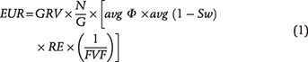
where GRV = gross rock volume, the product of the reservoir area × gross thickness; N/G = net-to-gross; Φ = effective porosity; Sw = water saturation; RE = recovery efficiency, the percentage of the in-place hydrocarbons ultimately recovered; and FVF = formation volume change factor for the hydrocarbons between reservoir and surface conditions. Oil shrinks, whereas gas expands.

The porosity, saturation, recovery efficiency, and 1/FVF can be multiplied to generate a recovery yield (RY). Therefore, the EUR equation can be simplified in two forms, each with three main components:

To provide clarity and consistency within an organization, the prospect’s EUR distribution represents success cases and should be determined before the assessment of the probability of geologic success (Pg).

The Pg is the chance of making a discovery equal to or exceeding the P99 EUR that would sustainably flow into the well from the penetrated target (Rose, 2001). That P99 can be approximated by the product of P90 values from each of the three main EUR input components noted above. Hence, Rose (2001) suggested that the chance of trap be assessed as the confidence that trap exists with at least the P90 area extent. Traditionally, the prospect Pg assumes a near-crestal well location such that the area updip of the location is less than the P90 of the productive area distribution. When determining the Pg, there is no consideration of commerciality of the resource—only the presence of hydrocarbons. The Pg equals the product of defined chance factors related to the petroleum system. Synonymous with chance of success Pwell and probability of success, Pg is expressed here as a percentage.

Minimum commercial field size (MCFS) is the field size that contributes to a discounted net present value (NPV) equal to zero, when burdened only with future development and operating costs, treating all prior investments as sunk. Ideally, a decision maker would approve the development of any discovery greater than the MCFS.

The probability of commercial success (Pc) = Pg × PMCFS, where PMCFS is, given a discovery, the chance of finding an EUR greater than or equal to the MCFS.

Next, Ptrap @ well is the percentile location on the area distribution that the area updip of the well location is found; it is synonymous with the phrase “area percentile.”

For Pwell = Pg × [(Ptrap @ well)/90%], Pwell is the chance that the downdip location will be a discovery. The denominator of 90% reflects the common standard that the trap chance factor is assessed as the chance of exceeding the P90 of the productive area distribution. For a well drilled at any location within the P90 productive area, the Ptrap @ well stays at 90%, so a prospect with a Pg = 50% has Pwell = 50% × [90%/90%] = 50%. For a prospect with a Pg = 50% but drilled at a location associated with P50 of the area distribution, Pwell = 50% × [50%/90%] = 28%.

The probability of commercial success for a well drilled downdip (Pwell (comm)) = Pwell × PMCFS (well) is the Pc for a well drilled downdip, where PMCFS (well) is the chance that a discovery at that downdip location will find an EUR greater than or equal to the MCFS.

Expected monetary value (EMV) is the sum of the probability-weighted NPVs (after tax) of commercial success and failure (where the NPV of commercial failure is negative). For any given commercial EUR case, the NPV is the discounted sum of each year’s net cash flow (income minus investment minus expense). Income is the revenue from producing the EUR. See the Appendix for more detail.

Example Prospect Details

Figure 1 illustrates a simple map and cross section for an example prospect used in the workflow. Before the application of the Pwell workflow, the prospect had its GRV generated from standard area versus depth plotting techniques (Frick and Taylor, 1962). Because this approach accurately captures the geometry of the trap, any correlation of the average net pay to the productive area is accounted for.

Figure 1. Example prospect and schematic cross section used for prospect assessment. The prospect has a probability of geological success of 50%, which incorporates a trap chance of 80%. The dotted contour encloses 300 ac, which is the 90th percentile of the productive area distribution. The vertical dashed line represents a well drilled with 400 ac updip from the location to the −5950-ft crest. The vertical dotted line represents a well location with 300 ac updip. Note how a discovery drilled at the 300-ac location could actually have a productive area closer to 400 ac due to the lower oil–water contact.

The area–depth pairs are plotted in Figure 2 for a simulation trial in which the gross reservoir thickness was 115 ft and the area was 400 ac. The oil-saturated GRV for this trial is the shaded closed polygon. The prospect has P90 and P10 gross reservoir thicknesses of 45 and 210 ft, respectively. For any trial, multiplication of the GRV by the N/G provides the net rock volume (NRV) and the average net pay is that NRV divided by the associated area.

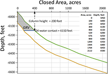Figure 2. Area versus depth below sea level plot for the example prospect used to generate the gross rock volume (GRV) (shaded polygon). In this trial, the GRV (31,844 ac-ft) includes a vertical reservoir gross thickness of 115 ft and an oil–water contact at −6150 ft such that the area equals the 400 ac discussed in Figure 1, with an associated hydrocarbon column height of 200 ft down from the crest.

The EUR distribution resulted from standard Monte Carlo techniques, in which each trial samples the input variable distributions and then multiplies them to create an EUR. The workflow used 20,000 trials. Ideally, all of the input parameters have undergone a reality checking process for distribution type and range. Figure 3 tabulates the prospect input parameter distributions summarized at the productive area, average net pay, and hydrocarbon recovery yield level, and tabulates and plots the output geologic and commercial EUR distributions on a log-probit plot.

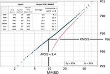Figure 3. Example prospect estimated ultimate recovery (EUR) distribution plotted in a log-probit coordinate system. Percentile values (P) for key inputs and output values shown in upper left corner. Recovery yield is defined in the text as the product of the volumetric parameters excluding the net rock volume. A minimum commercial field size (MCFS) of 9.4 million bbl of oil (MMBO) was applied to redistribute EUR values in excess of the MCFS as the curved “commercial distribution.” With a probability of geological success of 50% and the MCFS of 9.4 million bbl of oil that posts at P66, the probability of commercial success is 66% × 50% = 33%. Avg. = average; BO = barrels of oil; Pc = probability of commercial success; Pg = probability of geologic success; PMCFS = given a discovery, the chance of finding an EUR greater than or equal to the MCFS.

The vertical line represents the MCFS of 9.4 million bbl of oil (see the Appendix for determination details). The MCFS projects to P66 on the y axis, so 66% of the EUR outcomes exceed that threshold (PMCFS). Those outcomes have been redistributed to convey that only commercial outcomes would enable the project to move forward. This prospect has a Pg = 50%, and the probability of commercial success, Pc = Pg × PMCFS = 50% × 66% = 33%.

Traditionally, exploration prospects have been drilled at or near the crest; therefore, the numbers above would be appropriate for consideration. However, often there are business reasons to drill downdip of the P90 productive area on a trap. The following methodology is designed to quantify the response to important business-related questions pertinent to a noncrestal drill decision, in a clear and systematic fashion.

Methodology to Quantify Potential Downdip Locations

1. From the map, determine the area associated with the well location (AAWL). On the map in Figure 1, the potential location at the perimeter of the shaded area has an AAWL of 400 ac. The 400 ac plotted on the area distribution chart determines Ptrap @ well when projected to the vertical axis and is used to calculate Pwell (Figure 4).
2. For each trial:
   1. If the sampled area is less than the AAWL, then place that EUR value in the updip group. This assumes a dry hole at the well location.
   2. If the sampled area is greater than or equal to the AAWL, then place that EUR value in the downdip group. This assumes a discovery at the well location, which includes the discovered updip volume.
3. Repeat for n trials, sort by AAWL, record the percentiles, and calculate the mean for both EUR groups.
4. Calculate:
   1. Pwell (at AAWL) = Pg × [(% trials > AAWL)/90%]. The percentage of trials greater than or equal to the AAWL = Ptrap @ well.
   2. The percentage of trials in which EUR is greater than or equal to the MCFS for each of the updip and downdip groups.
5. Repeat these steps for other potential well locations to generate data for comparative valuation.

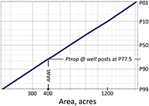Figure 4. Example prospect productive area distribution plotted in a log-probit coordinate system. The vertical line represents a 400-ac area associated with the well location (AAWL). This area posts at the 77.5th percentile (P77.5), which is used to generate the chance that the downdip location will be a discovery (Pwell) by applying the formula defined in the text. Ptrap @ well = percentile location on the area distribution that the area updip of the well location is found.

Figure 5 shows the unique workflow design for the methodology. Iterations of the workflow began at a well location 200 ac downdip from the prospect crest, then continued in increments of 100 ac, down to 1200 ac. These form the data set used for analysis, valuation, and discussion. Of note, for a discovery at any downdip location, the downdip EUR distribution represents the range of EUR from the prospect crest to the base of hydrocarbons in the well, plus the remaining EUR distribution from the base of the hydrocarbons in the well to the hydrocarbon water contact. Additional complexity—for example, incorporating a range of column heights—can be assessed using the techniques discussed in this paper.

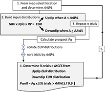Figure 5. Workflow map used to generate the chance the downdip location will be a discovery (Pwell) and updip and downdip estimated ultimate recovery (EUR) distributions. Gross rock volume (GRV), net-to-gross (N/G), and recovery yield (RY) represent the input distributions (GRV, N/G, and RY) defined in the text, which when multiplied generate the EUR distribution. In this simulation, n = 20,000 trials were computed for each specific downdip well location selected. A = productive area sampled in the simulation; AAWL = area associated with the well location; MCFS = minimum commercial field size; Pg = probability of geologic success.

RESULTS

The workflow in Figure 5 generated a set of Pwell and EUR results (Table 1). No commercial truncation has been applied. The trade-off between increasing EUR by drilling downdip and a lower chance of a discovery is displayed in Figure 6. As defined earlier, Pwell = Pg for locations within the P90 of the area distribution.

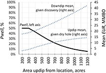Figure 6. Plot of chance the downdip location will be a discovery (Pwell ), on the left y axis for each downdip location shown decreasing, whereas the mean of the associated downdip and updip estimated ultimate recovery (EUR) distributions (right y axis) increase. MMBO = million barrels of oil.

A decision maker may ask, “Why not drill at the downdip area that generates the EUR of the MCFS?” Although this is a worthwhile question, the EUR is a function of many parameters, not just the area. Figure 7 plots the output EUR from 5000 of the 20,000-trial simulation against the input area. For example, although the 700-ac location is associated with a mean updip EUR just above the MCFS (Table 1), note the scatter of EUR values, with many less than the MCFS. A wide range of areal uncertainty can contribute to the MCFS, between 300 and 1200 ac. Large or small values for average net pay or the average porosity or recovery efficiency can contribute, often significantly, to the wide EUR range.

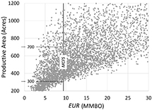Figure 7. Crossplot of productive area (acres) and resulting estimated ultimate recovery (EUR, millions of barrels of oil [MMBO]) for 5000 trials randomly selected from the 20,000-trial simulation. The vertical line is the minimum commercial field size (MCFS). Analysis of the 300- and 700-ac locations is described in the text.

Note that whenever 200 or 300 ac was selected in a trial, the resulting updip EUR was always less than the MCFS. Thus, a discovery at a location 200 or 300 ac downdip from the crest would likely require a downdip appraisal well to determine commerciality—hence, the importance of considering the full range of a location’s updip and downdip resources along with the associated chances of success in the decision-making process.

Table 2 illustrates the P99–P01 range of EUR values for the considered locations, and the associated probability metrics computed from the workflow and standard commercial truncation algebra.

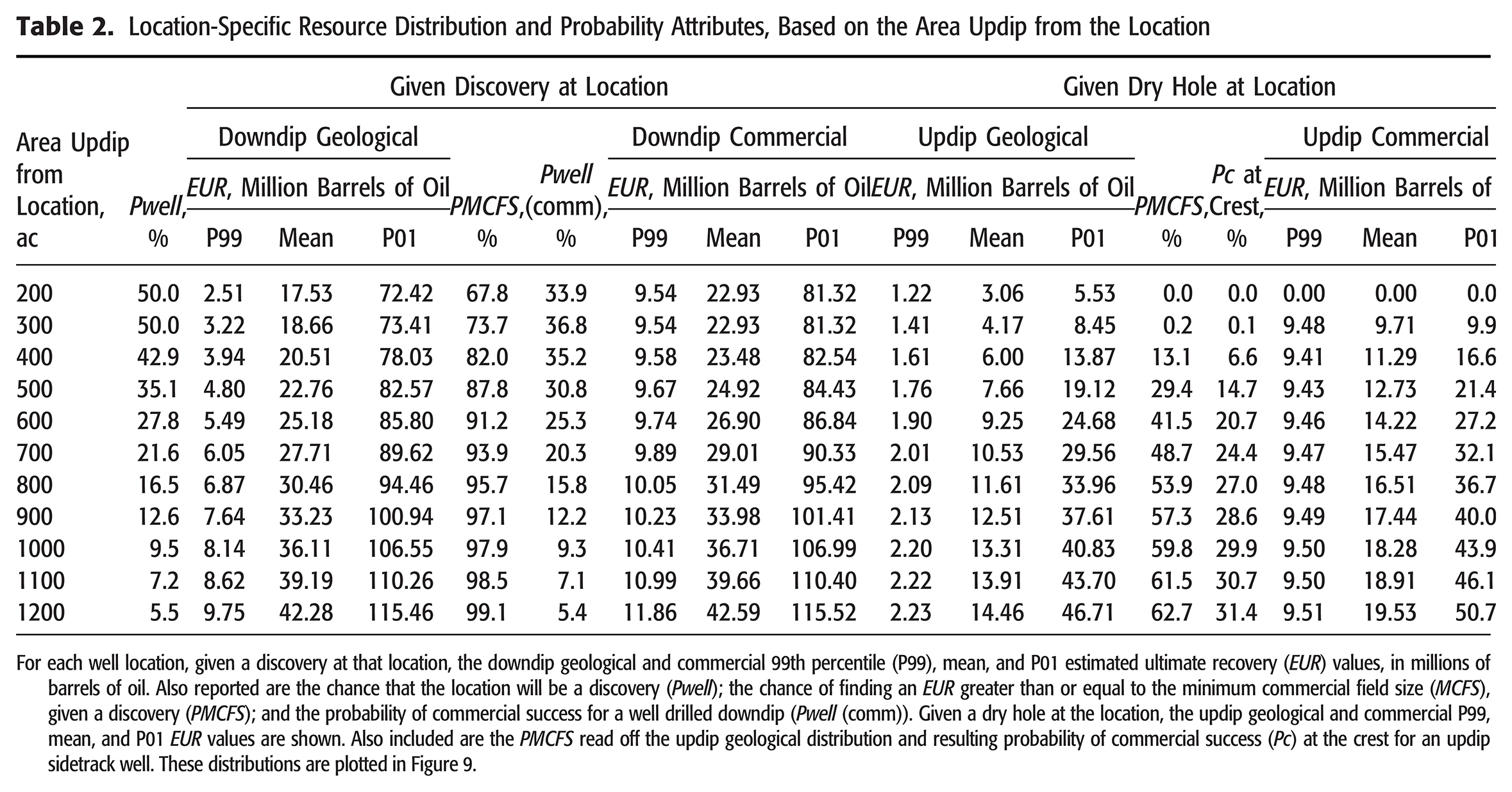
Figure 8 illustrates the splitting process that generates the updip and downdip EUR distributions for a well location with 400 ac updip. The MCFS of 9.4 million bbl of oil intersects the downdip EUR distribution, then projects to the y axis at P82. From Table 2, Pwell is 43%, so the Pwell (comm) = 82% ×43% = 35%.

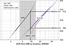Figure 8. Estimated ultimate recovery (EUR) distributions updip and downdip of a well location with 400 ac updip, plotted on a log-probit coordinate system, with the prospect probability of geologic success (Pg) = 50% and the chance the downdip location will be a discovery (Pwell) = 43%. The Pwell (comm) is the chance the downdip resources will be commercially successful, given the minimum commercial field size (MCFS) posts at the 82nd percentile (P82), such that Pwell (comm) = 82% × 43% = 35%. The commercial distribution associated with that is redistributed as the curved line. If the well location is a dry hole, then the MCFS can be projected to the updip resource distribution and projects at P13. Thus, given a dry hole, the probability of commercial success for a crestal well updip = 13% × Pg = 13% × 50% = 6.5%. The shaded rectangle represents the overlap of the updip and downdip distributions. MMBO = million barrels of oil; PMCFS = given a discovery, the chance of finding an EUR greater than or equal to the MCFS.

The EUR of the updip distribution has a P01 of approximately 14 million bbl of oil, a value that falls at approximately the P60 of the downdip geologic EUR distribution. The P99 EUR of the downdip distribution occurs at the P72 of the updip distribution. The degree of overlap of the updip and downdip distributions, which could be surprising to many, indicates the prevailing uncertainty. The amount of EUR overlap between the updip and downdip distributions will be a function of trap geometry, column height, and thickness variability. For example, for a stratigraphic trap wedge that thins to zero at the updip edge but thickens downdip, one would expect more separation between the downdip EUR distributions from the updip EUR distributions. In our example prospect, the RY parameters are the same for the updip and downdip trials so that only the GRV affects the EUR overlap.

Figure 9 plots the P99, P90, P50, P10, and P01 from the EUR distributions for the family of updip geologic distributions and the family of downdip geologic distributions for the locations considered. In the updip distributions, the upward deviation from (and above) perfectly straight lines (i.e., a lognormal distribution) results from the truncation effect that does not allow any areas greater than the location area. Once the MCFS is imposed on an EUR distribution, additional metrics related more to decision-making arise. Figure 10 shows how the commercial chance values can be further quantified and communicated for more informed decision-making. Curve 1 shows Pwell (comm) begins at 34% for the 200-ac location, increases slightly to a maximum value for the location associated with 300 ac, and then declines steadily. The peak at 300 ac is not seen on the Pwell curve (Figure 6) because the location is not beyond the P90 area, so the parameter Ptrap @ well is fixed at 100% and does not impact the calculation. However, the Pwell (comm) is derived from the Pwell times the percentage of downdip EUR outcomes greater than or equal to the MCFS (which steadily increases as the location moves downdip).

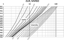Figure 9. Updip and downdip (dotted) estimated ultimate recovery (EUR) distributions for the 11 well locations assessed in 100-ac increments between 200 and 1200 ac. Each curve connects the 99th percentile (P99), P90, P50, P10, and P01 values of the distribution. See Table 2 for the P99, P01, and mean of each distribution. The downdip distributions represent the prospect crest to the base of hydrocarbons in the well, plus the remaining EUR distribution from the base of the hydrocarbons in the well to the hydrocarbon water contact, rather than being limited to that portion downdip of the location. MMBO = million barrels of oil.

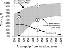Figure 10. The solid curve (1) represents the chance the potential well location will be a commercial discovery (Pwell (comm)). The shaded envelope has a lower bound (2) that represents for each location the chance, given a dry hole at that location, that there will be an updip commercial discovery. The upper bound (3) represents for each location, given a discovery there, the percent of the downdip estimated ultimate recovery (EUR) outcomes that exceed the minimum commercial field size (MCFS). Figure 8 shows those boundary values from the 400-ac location to be 13% and 82%, respectively. From a probability perspective, the larger the width of the shaded chance envelope, which reaches a maximum at 300 ac (4), the less ambiguous the well location decision is.

Figure 10 includes two other location-dependent metrics. First, given a dry hole, the chance that an updip discovery will exceed the MCFS (curve 2) is derived from the percentage of the trials that achieve that level when the oil column is limited to the well location (Table 2). This forms the bottom boundary of the shaded envelope, beginning at 0 for 200 ac and increases up to approximately 60% at 1200 ac downdip. For the 400-ac location detailed in Figure 8, note how the intersection of the MCFS with the updip EUR distribution is projected to approximately P13, contributing to the bottom part of the shaded envelope crossing 400 ac at 13%.

Second, given a discovery, the percentage of trials that generate an EUR greater than or equal to the MCFS (curve 3 in Figure 10) is the top of the shaded envelope, beginning at 68% for drilling 200 ac downdip. Figure 8 showed the MCFS intersection with the 400-ac location downdip EUR distribution projected to P82; hence, the upper part of the shaded envelope crosses 400 ac at 82%. Figure 9 showed that approximately 99% of the downdip EUR distribution associated with the most downdip (1200-ac) location exceeded the MCFS. This is corroborated by the area versus EUR crossplot (Figure 7), where at 1200 ac, all of the associated EUR values exceed the MCFS.

Third, the vertical arrow (4 in Figure 10) illustrates that the 300-ac location has the widest part of the shaded chance envelope. For a “perfect” well location, a discovery would have 100% chance of exceeding the MCFS, and a dry hole would leave the updip accumulation with 0% chance of exceeding the MCFS. In other words, a “perfect” well location would show no overlap of the updip and downdip EUR distributions. Thus, wider ranges in the shaded envelope between the “given discovery” and “given dry hole” chance curves are desired for the drilling well location. This maximum chance width at 300 ac coincides with the maximum Pwell (comm), can be considered the least ambiguous location, and deserves consideration in the valuation for the optimal location.

The rigorous workflow allows an exploration team to not only calculate the Pwell and Pwell (comm) as the well location moves downdip but also to probabilistically modify the prospect EUR distribution of a discovery to that well location as well as the updip “attic” resource potential. However, the valuation of the resources includes other parameters such as cost, timing, and productive rates. These factors lead to success case NPV values that can be probability weighted by commercial chance metrics to calculate which location generates the maximum EMV.

Valuation

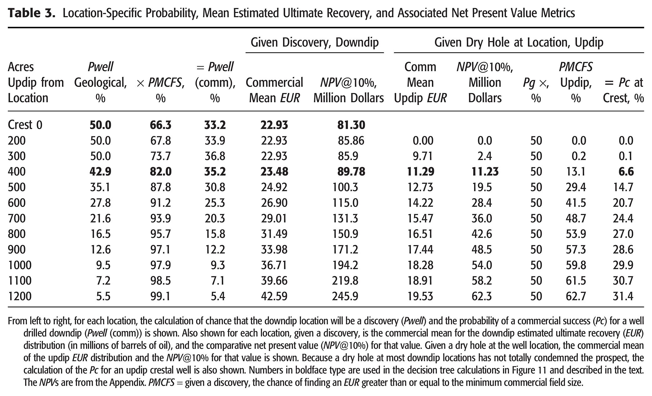
The trade-offs of increased resource potential downdip with a lower Pwell assist in the optimization of a well location through a decision tree analysis that can be solved for EMV. Haskett (2003) addressed building decision trees to assess appraisal drilling, focusing on how that information can ultimately reduce resource uncertainty. This current paper acknowledges the inevitable uncertainty for the decision maker and addresses comparative NPV (NPV@10%) of the mean commercial EUR associated with specific locations. The cash flow model of various development cases related to size, with associated salient details, are described in the Appendix. Table 3 summarizes key metrics from previous figures and tables with the NPV@10% for the commercial mean EUR to build a decision tree branch for valuation at each location. When the NPVs are properly probability weighted, the resulting EMV serves as valuable input to identify where unnecessary appraisal costs can be avoided.

For each case, the exploration well cost is $10 million. If required, an appraisal well costs $10 million and has an accompanying production delay of 0.5 yr, which further decreases the NPV. Different producing environments or supply conditions may dictate longer delays, which could be modeled easily and would further emphasize the benefit of identifying a well location that could eliminate the need for an appraisal well. As Figure 7 indicates, there is no unique productive area associated with the MCFS; consequently, a stepwise approach follows beginning with a base case drill location at the crest.

For each decision branch shown in Figure 11, the horizontal line at the far left is a primary branch and the number in the lower right corner (shaded box) is the EMV calculated. A circle represents a chance node, where the probabilities assigned to the adjacent branches must sum to 100%. The black squares after a discovery indicate the option to drill an appraisal well before development.

Figure 11. (A) Decision tree showing the expected monetary value (EMV) of drilling at the crest. The two black squares show that there is an option to drill a downdip appraisal well if there is a discovery (disc), which is pursued here. Note that this evaluation does not have a physical well location. The probabilities (Prob.) of the branches are based on the percent of the total number of simulation trials that exceed the minimum commercial field size (MCFS). (B) Decision tree for a location 400 ac downdip. The upper two black squares show that there is an option to drill a downdip appraisal well if there is a discovery, which is not pursued here. The lower black square indicates the option to drill an updip appraisal well if the location is a dry hole, but this is not pursued here. Estimated ultimate recovery (EUR), Prob., and net present value (NPV) from Table 3. (C) Decision tree for a location 400 ac downdip, where a discovery is followed by a downdip appraisal well, but a dry hole is not appraised with an updip appraisal well. The EUR, Prob., and NPV from Table 3. (D) Decision tree for a location 400 ac downdip, where a discovery is not followed by a downdip appraisal well. However, if the exploration well is a dry hole, then the circle represents the chance node an updip appraisal well will either succeed or fail. Comm. = commercial; expl = exploration; $MM = million dollars; MMBO = million barrels of oil; N = no; Pg = probability of geologic success; Pwell = chance that the downdip location will be a discovery; Y = yes.

The major decision branches that emanate from Figure 11A (crestal location) and continue with options for the 400-ac location (Figure 11B–D) are meant to assist in the decision-making process. The case with the highest EMV may not be pursued because management may not give approval for development if the EUR discovered with a lowest known oil in a reservoir is less than the MCFS. The risk tolerance of the decision maker is not addressed here, but it could alter the decision paths from the ones discussed below.

DISCUSSION

Figure 11A shows the tree for the crestal location, where a discovery is followed by a downdip appraisal well, readily justified because Figure 7 illustrates that there were no EUR values exceeding the MCFS until well locations had updip productive areas of 400 ac or more.

The prospect Pg is 50% and the PMCFS is 66.3%, generating a Pc = 33.2% (which becomes the probability weighting for the success branch); the resource valued is the mean commercial EUR, 22.3 million bbl of oil. The discounted cash flow model (with a 10% discount rate) generates a success case development NPV@10% of $81.3 million (see the Appendix). The NPV@10% for the success case outcome branch in Figure 11A is the development NPV@10%, including the exploration and appraisal costs and the startup delay of 0.5 yr due to the appraisal program. This adjustment is made using the standard time value of money equation (n = 0.5 yr appraisal delay; i = discount rate) less the exploration and appraisal well costs. As a result, the success case NPV@10% in millions of dollars is equal to

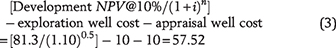
This generates an EMV (adding all probability weighted adjusted NPV@10% values from each end node) of $10.7 million, to which the other location (primary branch) valuations can be compared.

For each alternative downdip case, the approach is replicated with the appropriate size, chance, and NPVs from Table 3 to build a representative primary branch. Incorporated in the overall assessment is the fact that each branch can have specific options. For example, if the location results in a discovery less than MCFS, there is an option to drill a downdip appraisal well that burdens the discovery branch with appraisal capital and production time delay. If the location is a dry hole, then there is the option to drill an updip appraisal well, with the same burdens but applied to the valuation of the updip EUR distribution. The primary branch with the highest EMV suggests the path forward, but may not represent the best decision. Figure 11B–D illustrates some representative options for the 400-ac primary branch case.

Figure 11B shows the primary branch that models the decision of no appraisal well following either a discovery or a dry hole. With Pwell equal to 42.9% and PMCFS equal to 82% of the downdip EUR distribution, the Pwell (comm) is the branch probability of 43% × 82% = 35.2%. The downdip commercial mean EUR has increased to 23.5 million bbl of oil and generates a success case NPV@10% = $79.8 million and results in an EMV of $21.6 million.

Figure 11C illustrates executing the option to drill a downdip appraisal well in the event of a location discovery, but not to drill an updip appraisal well if the location is a dry hole. The success case NPV@10% = $65.62 million, which incorporates the exploration and appraisal wells and the associated production time delay. Notice that the appraisal well has a 18% chance of having EUR less than the MCFS, resulting in branch outcome with a $20 million loss. The options in this decision tree result in an EMV of $15.8 million, less than the $21.6 million EMV when the decision is to proceed directly to development. In other words, for this location, drilling an appraisal well predevelopment destroys value.

A third option models the decision not to drill a downdip appraisal well in the event of a discovery, but to include an updip appraisal well after a dry hole (Figure 11D). The end of the dry hole branch becomes a chance node to indicate the appraisal well will either be a discovery exceeding MCFS or a commercial failure, which could be a dry hole or discovery less than MCFS.

The discovery branch probability with EUR greater than or equal to the MCFS for the updip appraisal well is 6.6%, which after a dry hole is derived from Pg multiplied by PMCFS, or 50% × 13.1% = 6.6% (see Figure 8, in which the MCFS is applied to the updip EUR distribution). The original prospect Pg is used after a downdip dry hole (and would likely never increase, even assuming the reservoir and seal remain) because the Pg is designed to be associated with the P90 area, or smaller. Note that the branch with updip appraisal discovery with EUR greater than or equal to the MCFS has NPV@10% = −$9.3 million. This is because the development NPV@10% of $10.7 million did not cover the $20 million cost of drilling an exploration and appraisal well. However, it is developed because losing $9.3 million is better than losing $20 million if you do not develop it. The option in this decision tree result in EMV is $16.3 million. This value is preferable to the result of Figure 11C, but not the optimal case (Figure 11B), which avoids any appraisal drilling.

A fourth option (not shown in Figure 11) is to drill an appraisal well downdip in the event of a discovery and an appraisal well updip in the event of a dry hole. This path has the most cost burdens and thus the lowest EMV. Such an approach illustrates the importance of analyzing drilling options before the decision, and was applied to every location, with the results displayed in Figure 12. The gray curves in Figure 12 show the results of the four main options for appraisal wells applied uniformly to each location. The solid black curve represents the decision strategy by Pwell location from the available valid options. The letters A–D post the results from Figure 11A–D, respectively.

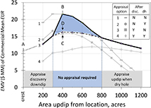Figure 12. The expected monetary value (EMV) versus well location area, with the cases indicated by letter (Figure 11A–D). Each of the gray curves represent whether a downdip appraisal is drilled after a discovery (disc.), and whether an updip appraisal is drilled after a dry hole (dh). The shaded polygon represents location areas with enhancement of EMV by saving appraisal costs. EUR = estimated ultimate recovery; $MM = million dollars.

Figure 7 demonstrates that no EUR values greater than the MCFS were generated from locations with 300 ac or less updip; therefore, a discovery at one of these locations should prompt a downdip appraisal well (option path 3). This is tantamount to saying that discoveries at these locations likely confirm only very small column heights relative to the 550-ft maximum column available.

For locations from 400 to 700 ac downdip, discoveries indicate a larger column with progressively larger amounts of EUR in excess of the MCFS, so no appraisal is required (Figure 12, option path 1), saving costs and maximizing EMV without the previous concerns of a minimal resource. Option path 2, where there would be an updip appraisal well given a dry hole at those locations, represents the second-best option; therefore, the shaded area highlights the incremental value created from the optimizing strategy.

For locations 800 ac downdip to the spill point, any discoveries would document an extensive column relative to the maximum possible column so that no further downdip appraisal would be needed. A dry hole at any of these locations should warrant consideration for an updip appraisal well (option path 2) because there could be large attic resources available. However, a decision maker may consider these locations to be far too downdip for the initial exploration well because Pwell values are less than 20% (Figure 6).

In summary, this workflow demonstrated that the 400-ac location with no appraisal wells was the optimal case based on a key decision metric (EMV). Other critical factors for the locations, moving downdip are as follows.

1. Locations encompassing 200 and 300 ac, given a dry hole, cannot support an updip appraisal well because the updip EUR distributions are entirely below the MCFS of 9.4 million bbl of oil (Figures 7, 9).
2. A well location between 400 and 500 ac downdip decreases Pwell from 50% to 40%, with Pwell (comm) decreasing from 35% to 30% (Figures 6, 10). This same location range is associated with a 20%–30% chance of leaving behind updip commercial resources. The trade-off is that a discovery at these locations provides an 80%–90% chance of a commercial accumulation (Figure 10).
3. For well locations 400–600 ac downdip, the P90 downdip resources for a discovery are close to or greater than the MCFS (Figure 9). Given a dry hole, the Pc for a sidetrack to test the crest from the 400-ac location would be 7% (and 21% from the 600-ac location). If that updip test is a discovery, then the mean resources would be 6.0 million bbl of oil at 400 ac and 9.2 million bbl of oil at 600 ac, each below the MCFS of 9.4 million bbl of oil.

CONCLUSIONS

Traditional consideration of a prospect for drilling requires the characterization of the full range of prospect EUR, associated chance of geologic success, and knowledge of a MCFS for valuation metrics. However, when considering drilling potential downdip locations, additional analyses can illustrate the updip and downdip resources for each location, as well as the associated chance that the location will be geologically and commercially successful. The trade-offs of decreased chance associated with increased resources can be illustrated and structured in a decision tree format. Such an approach quantifies the consequences of decisions before investment. Drilling a location where EMV is maximized, due to the ability to eliminate an appraisal well downdip to confirm commerciality or updip to chase potential left-behind resources, can now be clearly characterized and communicated for more informed decision making.

APPENDIX: CALCULATION OF NPVs

Using standard discounted cash flow analysis, multiple development cases were calculated to estimate the MCFS and a range of NPV@10% that covered the EUR distribution. In addition to the MCFS case of 9.4 million bbl of oil (the EUR generating NPV@10% = 0), this approach generated an NPV@10% for the following EUR (million bbl of oil): 3.5, 15.0, 22.3, 30.0, 50.0, and 72.1.

All of the development cases assumed that all of the wells were drilled in the first year, with production startup the following year. The number of producers were based on an 80-ac well spacing applied to the area that is representative of that EUR being developed. Initial well rates were based on a productivity index of approximately 14 BOPD/ft of average net pay. Production forecasts were based on an exponential production decline rate varying from 19%/yr for the smallest noncommercial case to 13%/yr for the largest case. The production plot for all of the cases is shown in Figure 13.

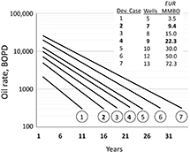Figure 13. Production profiles (oil rate in BOPD versus year) that contribute to the income cash flow stream for the seven development cases. Development (Dev.) case 1, which produces 3.5 million bbl of oil (MMBO) from five wells, is below the minimum commercial field size of 9.4 MMBO shown by case 2 and deemed noncommercial. The cash flow details for cases 2 and 4 are shown in Figure 14. EUR = estimated ultimate recovery.

Capital expenses of $10 million per development well and facilities costs ranging from $20 to $83 million were applied in year 1. The operating expenses to support this production varied from $11.10/bbl of oil for the smallest EUR case to $6.00/bbl of oil for the largest EUR case. The price of oil was kept constant at $50/bbl of oil. The cash flow streams were modeled to the economic limit, with producing life for the developed cases ranging from 16 to 34 years.

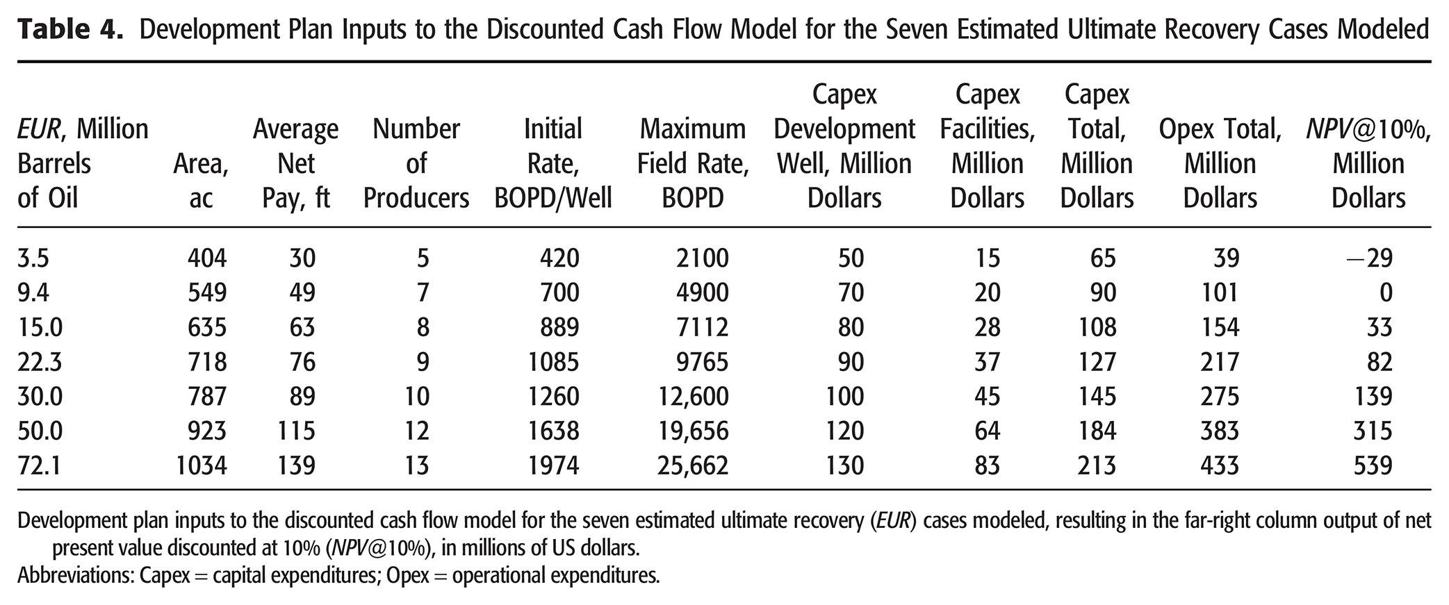
The resulting net cash flow stream with a 50% tax rate was discounted at a 10% discount rate using the mid-year discounting method to calculate the cumulative NPV (NPV@10%) for each development case. Salient information from each case is summarized in Table 4.

The annual cash flow streams for the 9.4 and 22.3 million bbl of oil cases are shown in Figure 14. The results from each NPV@10% calculation was plotted against the input EUR, and a polynomial curve was applied to best fit the data points. This enabled an accurate estimate of NPV@10% for any simulated commercial EUR output associated with the various downdip drilling locations (Figure 15). These development NPV@10% values were then adjusted to include the exploration well cost and the appraisal well cost, if any. If an appraisal well was drilled, then the production start-up was delayed 6 months, with the associated time value of money reduction applied. The success case NPV@10% values shown in the decision trees includes all of these adjustments, as appropriate, for each outcome branch.

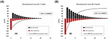Figure 14. Annual net revenue, total expenses, and cumulative (Cum) net cash flow for (A) development case 2 (estimated ultimate recovery [EUR] = 9.4 million bbl of oil [MMBO]) and (B) development case 4 (EUR = 22.3 MMBO). The 9.4 MMBO produced in case 2 generates a comparative net present value (NPV@10%) = 0, defining the minimum commercial field size. $MM = million dollars.

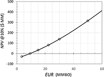Figure 15. Development comparative net present value (NPV@10%) versus estimated ultimate recovery (EUR) curve built as a polynomial best fit to seven cases shown in Figure 13 (only the six smallest cases shown). This curve is before the impact of exploration and appraisal costs, and the time value of production delay in the case of appraisal. $MM = million dollars; MMBO = million barrels of oil.

REFERENCES CITED

Capen, E. C., 1976, The difficulty of assessing uncertainty: Journal of Petroleum Technology, v. 28, no. 8, p. 843–850, doi:10.2118/5579-PA.
Citron, G. P., P. J. Brown, J. Mackay, P. Carragher, and D. Cook, 2018, The challenge of unbiased application of risk analysis towards future profitable exploration, in M. Bowman and B. Levell, eds., Petroleum geology of NW Europe: 50 years of learning: Geological Society, London, Petroleum Geology Conference Series, v. 8, p. 259–266, doi:10.1144/PGC8.2.
Frick, T. C., and R. W. Taylor, 1962, Petroleum production handbook, v. II, Reservoir engineering: New York, McGraw-Hill, 432 p.
Haskett, W. J., 2003, Optimal appraisal well location through efficient uncertainty reduction and value of information techniques: Society of Petroleum Engineers Annual Technical Conference and Exhibition, Denver, Colorado, October 5–8, 2003, SPE-84241-MS, doi:10.2118/84241-MS.
Milkov, A. V., 2015, Risk tables for less biased and more consistent estimation of probability of geological success (PoS) for segments with conventional oil and gas prospective resources: Earth-Science Reviews, v. 150, no. 11, p. 453–476, doi:10.1016/j.earscirev.2015.08.006.
Milkov, A. V., 2021, Reporting the expected exploration outcome: When, why and how the probability of geological success and success-case volumes for the well differ from those for the prospect: Journal of Petroleum Science and Engineering, v. 204, 108754, 8 p., doi:10.1016/j.petrol.2021.108754.
Otis, R. M., and P. Haryott, 2010, Calibration of uncertainty (P10-P90) in exploration prospects: AAPG Annual Convention and Exhibition, New Orleans, Louisiana, April 11–14, 2010, 23 p., accessed March 20, 2023, https://www.searchanddiscovery.com/pdfz/documents/2010/40609otis/ndx_otis.pdf.html.
Otis, R. M., and N. Schneidermann, 1997, A process for evaluating exploration prospects: AAPG Bulletin, v. 81, no. 7, p. 1087–1109, doi:10.1306/522B49F1-1727-11D7-8645000102C1865D.
Quirk, D. G., and R. G. Ruthrauff, 2008, Toward consistency in petroleum exploration: A systematic way of constraining uncertainty in prospect volumetrics: AAPG Bulletin, v. 92, no. 10, p. 1263–1291, doi:10.1306/06040808064.
Rose, P. R., 2001, Risk analysis and management of petroleum exploration ventures: AAPG Methods in Exploration Series 12, 164 p., doi:10.1306/Mth12792.
Schneider, M., and D. Cook, 2017, Drilling a downdip location: Effect on updip and downdip resource estimates and commercial chance: AAPG Search and Discovery article 42102, accessed May 21, 2021, http://www.searchanddiscovery.com/pdfz/documents/2017/42102schneider/ndx_schneider.pdf.html.
AUTHORS
Mark Schneider is a partner with Rose & Associates. He is active in consulting, training, and software focusing on risk analysis and uncertainty characterization of upstream opportunities. He received a B.S. degree in chemical engineering and a B.S. degree in natural gas engineering from Texas A&I University in 1981. He received an M.S. degree in petroleum engineering from the University of Houston in 1991.
Gary P. Citron is a senior associate with Rose & Associates and served as managing partner from 2003 to 2014. In 2008, he co-founded the Risk Coordinators Workshop, which continues today. From 1994 to 1998 he served on Amoco’s assurance team. He received his B.S. degree in geology from the University at Buffalo and his Ph.D. in geology from Cornell University. He is the corresponding author of this paper.
Paul Haryott is a principal consultant with Rose & Associates. He has led assurance teams and been a senior manager in major oil companies and has a special interest in new opportunity development and exploration management. He received his B.Sc. degree in geology from Liverpool University in 1996 and his M.Sc. degree in petroleum exploration studies from Aberdeen University in 1997.
David Cook is a partner at Rose & Associates and the manager of their software company. He has led the development of prospect, play, and portfolio risk analysis tools since 2004 and implemented the Pwell functionality in the RoseRA prospect assessment software. He received his B.S. degree in geophysics from Texas A&M University in 1978 and worked at Mobil Oil until 2000.
ACKNOWLEDGMENTS
We thank Peter Carragher and Doug Weaver (both with Rose & Associates) for their encouragement and critical reviews before the submission of this paper. We also thank the AAPG editors for their improvements to the paper. Rose & Associates’ RoseRA prospect assessment software performed the calculations and provided the results following the workflow provided.